 DALI bias#
Systematic differences between observed data and a model can shift inferred parameters. Fisher bias predicts these shifts using a linear approximation around the fiducial parameters. For nonlinear models, however, the parameter response can depart substantially from this prediction.
DALI bias extends Fisher bias by retaining higher-order derivatives of the model. It provides predictions for shifts in both the maximum a posteriori (MAP) estimator and the posterior mean. The underlying formalism and its numerical validation are presented in Šarčević, Van der Wild et al. (2026).
This example illustrates Fisher and DALI bias calculations using a two-parameter nonlinear model with a non-Gaussian posterior.
Nonlinear model and systematic mismatch#
Model definition#
We consider two parameters, \(\boldsymbol{\theta}=(u,v)\), and two observables,
where \(\Delta u=u-u_0\), \(\Delta v=v-v_0\), and
The first observable provides a broad constraint on the parameters, while the second constrains a curved parameter combination. We assume a fixed covariance with fractional errors of 10% and a correlation coefficient of 0.3.
>>> import numpy as np
>>> from derivkit import ForecastKit
>>> theta0 = np.array([0.15, 0.05])
>>> def model(theta):
...     u, v = theta
...     du = u - theta0[0]
...     dv = v - theta0[1]
...     return np.array([
...         1.0 + 1.4 * du + 0.15 * dv
...         + 0.20 * du**2 + 0.06 * du * dv,
...         0.8 + 10.0 * (
...             dv + 1.8 * du**2 - 0.3 * du**3
...             + 0.20 * du * dv
...         ),
...     ])
>>> sigma = 0.10 * np.abs(model(theta0))
>>> correlation = np.array([[1.0, 0.3], [0.3, 1.0]])
>>> cov = np.outer(sigma, sigma) * correlation
>>> fk = ForecastKit(function=model, theta0=theta0, cov=cov)
The nonlinear dependence of the observables produces a curved posterior geometry that is not generally captured by a Gaussian approximation.
Systematic displacement#
We introduce an additive systematic displacement in data space,
where \(A\) controls the systematic amplitude.
The model used for inference remains unchanged. The systematic modifies only the data vector, allowing us to study the resulting parameter shift.
For the following calculations, we choose \(A=10\).
>>> amplitude = 10.0
>>> systematic = np.array([0.020, -0.003])
>>> data_unbiased = model(theta0)
>>> data_biased = data_unbiased + amplitude * systematic
>>> dn = fk.delta_nu(
...     data_unbiased=data_unbiased,
...     data_biased=data_biased,
... )
>>> print(np.round(dn, 3))
[ 0.2  -0.03]
Systematic bias tensors#
Fisher bias#
Fisher bias provides the first-order prediction for the parameter shift induced by a systematic displacement. Its formalism and implementation are described in the Fisher bias example.
Here, we use Fisher bias as a reference for assessing the nonlinear corrections introduced by DALI.
DALI bias#
DALI generalizes the Fisher calculation by retaining higher derivatives of the model. The systematic bias tensors are
The first-order tensor corresponds to the Fisher bias vector. Higher-order tensors describe how the systematic couples to the nonlinear model response.
We calculate the bias tensors up to and including third derivative order.
The bias_order argument specifies the highest model derivative order,
equivalently the number of parameter indices of the bias tensors, rather
than the order of the expansion in systematic amplitude.
Here, bias_order=3 matches the third-order DALI forecast.
>>> bias = fk.dali_bias_tensor(
...     delta_nu=dn,
...     bias_order=3,
... )
>>> sorted(bias)
[1, 2, 3]
The corresponding unbiased DALI forecast tensors can be obtained independently:
>>> dali = fk.dali(forecast_order=3)
>>> sorted(dali)
[1, 2, 3]
Together, these tensors describe the nonlinear posterior geometry and its response to the systematic displacement.
Parameter shifts#
MAP shift#
The MAP shift describes how the maximum of the posterior moves when the systematic is introduced.
DALI expands this response in successive orders of the systematic amplitude,
The first-order contribution reproduces Fisher bias, while the higher-order contributions account for nonlinear corrections.
>>> fisher = fk.fisher()
>>> _, fisher_shift = fk.fisher_bias(
...     fisher_matrix=fisher,
...     delta_nu=dn,
... )
>>> map_shift, map_metadata = fk.dali_map_shift(
...     delta_nu=dn,
...     expansion_order=3,
...     return_metadata=True,
... )
>>> sorted(map_metadata["terms"])
[1, 2, 3]
The metadata separates the individual response orders:
print("Fisher shift:", fisher_shift)
print("DALI MAP shift:", map_shift)

for order, term in map_metadata["terms"].items():
    print(f"Order {order}:", term)
The predicted biased MAP is also available as
map_metadata["estimator"].
Posterior mean shift#
For a non-Gaussian posterior, the MAP and posterior mean generally differ. The systematic shift of the posterior mean is defined as
DerivKit provides an analytic approximation using a local expansion around the MAP.
>>> mean_shift, mean_metadata = fk.dali_mean_shift(
...     delta_nu=dn,
...     return_metadata=True,
... )
The metadata contains the predicted baseline and biased posterior means.
print("Unbiased mean:", mean_metadata["baseline"])
print("Biased mean:", mean_metadata["estimator"])
print("Mean shift:", mean_shift)
Unlike the MAP shift, the posterior mean shift is not generally equal to the displacement of the biased mean from \(\boldsymbol{\theta}_0\).
Posterior mean response#
An alternative approach expands the posterior mean directly around the unbiased reference posterior.
The method uses samples or integration nodes representing that posterior. Here, we use deterministic integration nodes weighted by the unbiased posterior density to accurately evaluate the response coefficients.
>>> axis_u = np.linspace(-0.5, 0.8, 151)
>>> axis_v = np.linspace(-0.5, 0.8, 151)
>>> uu, vv = np.meshgrid(axis_u, axis_v, indexing="ij")
>>> nodes = np.column_stack([uu.ravel(), vv.ravel()])
>>> predictions = np.array([model(theta) for theta in nodes])
>>> inv_cov = np.linalg.inv(cov)
>>> residual = data_unbiased - predictions
>>> chi2 = np.einsum("ni,ij,nj->n", residual, inv_cov, residual)
>>> weights = np.exp(-0.5 * (chi2 - chi2.min()))
The integration weights represent the unbiased posterior density. For a uniform grid, the common integration cell area cancels when the weights are normalized.
>>> response_shift, response_metadata = fk.dali_mean_response(
...     delta_nu=dn,
...     theta=nodes,
...     weights=weights,
...     forecast_order=3,
...     response_order=4,
...     return_metadata=True,
... )
The response expansion can be evaluated up to fourth order in
systematic amplitude. The individual contributions are available
in response_metadata["terms"].
Unlike the local analytic approximation,
derivkit.forecast_kit.ForecastKit.dali_mean_response()
retains the full unbiased DALI posterior as its reference
distribution and expands only its response to the systematic.
For this benchmark, the cubic model is reproduced exactly by the third-order DALI expansion. The remaining error in the response prediction therefore arises from truncating the systematic amplitude expansion and from numerical integration.
Posterior visualization#
We compare the unbiased and biased Fisher and DALI posteriors. The Fisher approximation describes a Gaussian posterior whose mean shifts in response to the systematic displacement, while its covariance remains unchanged.
The DALI approximation retains the nonlinear posterior geometry.
Both DALI posteriors are sampled using
derivkit.forecast_kit.ForecastKit.getdist_dali_emcee(),
with the systematic bias tensors included only in the biased posterior.
import numpy as np
from getdist import plots
from derivkit import ForecastKit

theta0 = np.array([0.15, 0.05])

def model(theta):
    u, v = theta
    du = u - theta0[0]
    dv = v - theta0[1]
    return np.array([
        1.0 + 1.4 * du + 0.15 * dv
        + 0.20 * du**2 + 0.06 * du * dv,
        0.8 + 10.0 * (
            dv + 1.8 * du**2 - 0.3 * du**3
            + 0.20 * du * dv
        ),
    ])

sigma = 0.10 * np.abs(model(theta0))
correlation = np.array([[1.0, 0.3], [0.3, 1.0]])
cov = np.outer(sigma, sigma) * correlation

fk = ForecastKit(function=model, theta0=theta0, cov=cov)

amplitude = 10.0
systematic = np.array([0.020, -0.003])
dn = amplitude * systematic

# Fisher forecast and systematic bias.
fisher = fk.fisher()
fisher_bias_vector, fisher_shift = fk.fisher_bias(
    fisher_matrix=fisher,
    delta_nu=dn,
)

# DALI forecast and systematic bias tensors.
dali = fk.dali(forecast_order=3)
bias = fk.dali_bias_tensor(
    delta_nu=dn,
    bias_order=3,
)

# Unbiased Fisher posterior.
posterior_fisher_unbiased = fk.getdist_fisher_gaussian(
    fisher=fisher,
    names=["u", "v"],
    labels=["u", "v"],
    label="Unbiased Fisher",
)

# Biased Fisher posterior.
posterior_fisher_biased = fk.getdist_fisher_gaussian(
    fisher=fisher,
    bias=fisher_bias_vector,
    names=["u", "v"],
    labels=["u", "v"],
    label="Biased Fisher",
)

# Unbiased DALI posterior.
posterior_dali_unbiased = fk.getdist_dali_emcee(
    dali=dali,
    names=["u", "v"],
    labels=["u", "v"],
    forecast_order=3,
    label="Unbiased DALI",
)

# Biased DALI posterior.
posterior_dali_biased = fk.getdist_dali_emcee(
    dali=dali,
    bias=bias,
    names=["u", "v"],
    labels=["u", "v"],
    forecast_order=3,
    label="Biased DALI",
)

# DerivKit color palette.
dk_blue = "#3b9ab2"
dk_yellow = "#e1af00"
dk_red = "#f21901"
line_width = 1.5

plotter = plots.get_subplot_plotter(width_inch=3.6)
plotter.settings.linewidth_contour = line_width
plotter.settings.linewidth = line_width
plotter.settings.figure_legend_frame = False

plotter.triangle_plot(
    [
        posterior_fisher_unbiased,
        posterior_fisher_biased,
        posterior_dali_unbiased,
        posterior_dali_biased,
    ],
    params=["u", "v"],
    legend_labels=[
        "Unbiased Fisher",
        "Biased Fisher",
        "Unbiased DALI",
        "Biased DALI",
    ],
    legend_ncol=1,
    filled=[False, False, False, False],
    contour_colors=[dk_blue, dk_blue, dk_yellow, dk_red],
    contour_ls=["--", "-", "-", "-"],
)
(png)
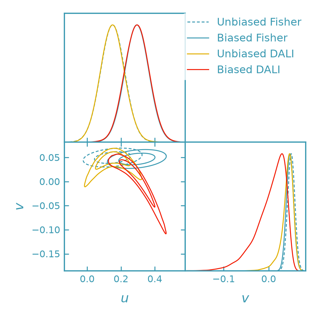
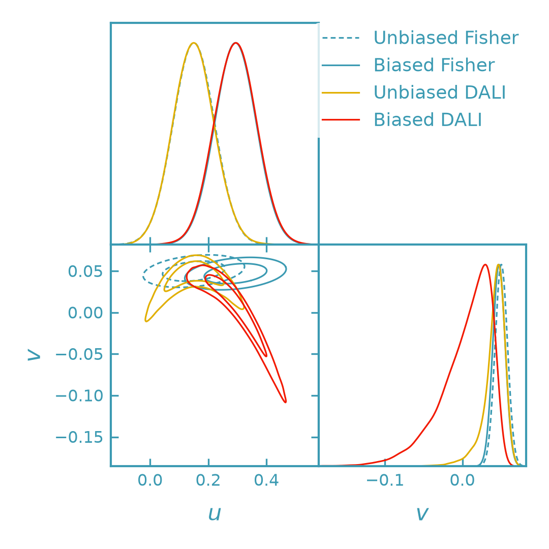
The dashed blue and solid yellow contours represent the unbiased Fisher and DALI posteriors, respectively. The solid blue and red contours show their corresponding biased posteriors.
Fisher bias translates the Gaussian posterior without changing its covariance. DALI bias instead modifies the nonlinear posterior through higher-order systematic response terms.
Systematic amplitude dependence#
To explore the nonlinear response, we vary the systematic amplitude from \(A=0\) to \(A=20\).
For each amplitude, we compare the Fisher prediction, the DALI MAP prediction, and the MAP obtained by minimizing the full nonlinear likelihood.
import numpy as np
import matplotlib.pyplot as plt
from scipy.optimize import minimize
from derivkit import ForecastKit

theta0 = np.array([0.15, 0.05])

def model(theta):
    u, v = theta
    du = u - theta0[0]
    dv = v - theta0[1]
    return np.array([
        1.0 + 1.4 * du + 0.15 * dv
        + 0.20 * du**2 + 0.06 * du * dv,
        0.8 + 10.0 * (
            dv + 1.8 * du**2 - 0.3 * du**3
            + 0.20 * du * dv
        ),
    ])

sigma = 0.10 * np.abs(model(theta0))
correlation = np.array([[1.0, 0.3], [0.3, 1.0]])
cov = np.outer(sigma, sigma) * correlation
inv_cov = np.linalg.inv(cov)

fk = ForecastKit(function=model, theta0=theta0, cov=cov)
fisher = fk.fisher()

systematic = np.array([0.020, -0.003])
amplitudes = np.linspace(0.0, 20.0, 21)

fisher_shifts = []
dali_shifts = []
exact_shifts = []

for amplitude in amplitudes:
    dn = amplitude * systematic

    _, fisher_shift = fk.fisher_bias(
        fisher_matrix=fisher,
        delta_nu=dn,
    )

    dali_shift = fk.dali_map_shift(
        delta_nu=dn,
        expansion_order=3,
    )

    data = model(theta0) + dn

    def negative_loglike(theta):
        residual = data - model(theta)
        return residual @ inv_cov @ residual

    result = minimize(negative_loglike, theta0, method="BFGS")

    fisher_shifts.append(fisher_shift)
    dali_shifts.append(dali_shift)
    exact_shifts.append(result.x - theta0)

fisher_shifts = np.asarray(fisher_shifts)
dali_shifts = np.asarray(dali_shifts)
exact_shifts = np.asarray(exact_shifts)

dk_yellow = "#e1af00"
dk_red = "#f21901"
dk_dark = "#555555"
line_width = 1.5

fig, axes = plt.subplots(1, 2, figsize=(7.2, 3.0))

for i, ax in enumerate(axes):
    ax.plot(
        amplitudes,
        fisher_shifts[:, i],
        "--",
        color=dk_dark,
        linewidth=line_width,
        label="Fisher",
    )
    ax.plot(
        amplitudes,
        dali_shifts[:, i],
        "-",
        color=dk_yellow,
        linewidth=line_width,
        label="DALI MAP",
    )
    ax.plot(
        amplitudes,
        exact_shifts[:, i],
        "o",
        color=dk_red,
        markersize=3,
        label="Numerical MAP",
    )

    ax.set_xlabel("Systematic amplitude $A$")
    ax.set_ylabel(
        r"$\Delta u$" if i == 0 else r"$\Delta v$"
    )

axes[0].legend(frameon=False)
fig.tight_layout()
plt.show()
(png)
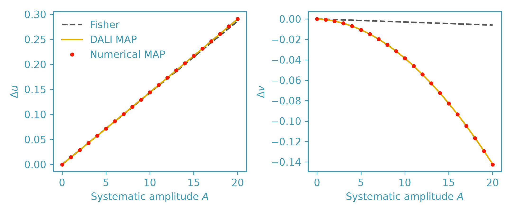
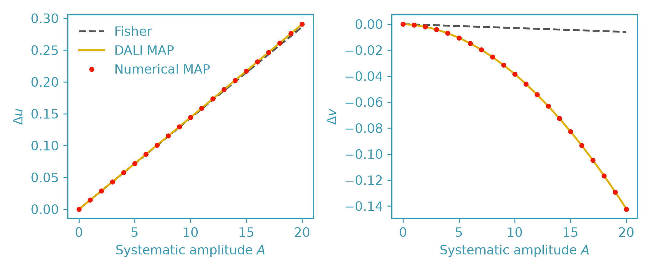
The Fisher prediction is linear in the systematic amplitude, while the DALI prediction includes higher-order corrections. The numerical MAP provides a reference for the full nonlinear model.
Numerical comparison#
The accuracy of the DALI predictions can be assessed by comparing them with direct inference using the original nonlinear model.
For the MAP, we minimize the negative log likelihood. For the posterior mean, we integrate the corresponding posterior over parameter space.
The following example compares Fisher bias, the DALI MAP shift, and both DALI posterior mean approximations with their numerical references.
import numpy as np
from scipy.optimize import minimize
from derivkit import ForecastKit

theta0 = np.array([0.15, 0.05])

def model(theta):
    u, v = theta
    du = u - theta0[0]
    dv = v - theta0[1]
    return np.array([
        1.0 + 1.4 * du + 0.15 * dv
        + 0.20 * du**2 + 0.06 * du * dv,
        0.8 + 10.0 * (
            dv + 1.8 * du**2 - 0.3 * du**3
            + 0.20 * du * dv
        ),
    ])

sigma = 0.10 * np.abs(model(theta0))
correlation = np.array([[1.0, 0.3], [0.3, 1.0]])
cov = np.outer(sigma, sigma) * correlation
inv_cov = np.linalg.inv(cov)

fk = ForecastKit(function=model, theta0=theta0, cov=cov)

amplitude = 10.0
systematic = np.array([0.020, -0.003])
dn = amplitude * systematic

data_unbiased = model(theta0)
data_biased = data_unbiased + dn

fisher = fk.fisher()

_, fisher_shift = fk.fisher_bias(
    fisher_matrix=fisher,
    delta_nu=dn,
)

map_shift = fk.dali_map_shift(
    delta_nu=dn,
    expansion_order=3,
)

local_mean_shift = fk.dali_mean_shift(delta_nu=dn)

# Deterministic integration grid.
axis_u = np.linspace(-0.5, 0.8, 151)
axis_v = np.linspace(-0.5, 0.8, 151)
uu, vv = np.meshgrid(axis_u, axis_v, indexing="ij")
nodes = np.column_stack([uu.ravel(), vv.ravel()])
predictions = np.array([model(theta) for theta in nodes])

def posterior_weights(data):
    residual = data - predictions
    chi2 = np.einsum(
        "ni,ij,nj->n",
        residual,
        inv_cov,
        residual,
    )
    return np.exp(-0.5 * (chi2 - chi2.min()))

weights0 = posterior_weights(data_unbiased)
weights1 = posterior_weights(data_biased)

# DALI posterior mean response.
response_mean_shift = fk.dali_mean_response(
    delta_nu=dn,
    theta=nodes,
    weights=weights0,
    forecast_order=3,
    response_order=4,
)

# Numerical posterior mean shift.
mean0 = np.average(nodes, axis=0, weights=weights0)
mean1 = np.average(nodes, axis=0, weights=weights1)
exact_mean_shift = mean1 - mean0

# Numerical MAP shift.
def objective(theta):
    residual = data_biased - model(theta)
    return residual @ inv_cov @ residual

exact_map_shift = (
    minimize(objective, theta0, method="BFGS").x - theta0
)

print("Fisher shift:", fisher_shift)
print("DALI MAP shift:", map_shift)
print("Numerical MAP shift:", exact_map_shift)
print()
print("Local DALI mean shift:", local_mean_shift)
print("DALI mean response:", response_mean_shift)
print("Numerical mean shift:", exact_mean_shift)
The numerical results for this example are:
Fisher shift: [ 0.14317857 -0.003     ]
DALI MAP shift: [ 0.14424626 -0.03841198]
Numerical MAP shift: [ 0.14424137 -0.03844078]

Local DALI mean shift: [ 0.14306221 -0.04524528]
DALI mean response: [ 0.14429223 -0.03719802]
Numerical mean shift: [ 0.14429211 -0.03719397]
The DALI MAP prediction closely follows the numerical MAP, including the nonlinear shift in the second parameter that is missed by Fisher bias.
For the posterior mean, the fourth-order response approximation agrees with numerical integration to an absolute Euclidean error of approximately \(4.1\times10^{-6}\) at \(A=10\). This comparison isolates the response expansion error at the chosen integration resolution.
The MAP and posterior mean are distinct estimators and should be compared separately. The accuracy of either DALI approximation depends on the posterior geometry and the magnitude of the systematic displacement.