Gaussian Fisher matrix#

This section shows how to compute a Gaussian Fisher matrix for models with a parameter-dependent mean and, optionally, a parameter-dependent covariance.

The Gaussian Fisher generalizes the standard Fisher matrix by including contributions from derivatives of the covariance matrix when \(C(\theta)\) depends on the model parameters.

For a model with mean prediction \(\mu(\theta)\) and covariance \(C(\theta)\), the Fisher matrix is

\[F_{\alpha\beta} = \mu_{,\alpha}^{\mathrm T} C^{-1} \mu_{,\beta} + \frac{1}{2} \mathrm{Tr}\!\left[ C^{-1} C_{,\alpha} C^{-1} C_{,\beta} \right].\]

If the covariance is independent of the parameters, the second term vanishes and the expression reduces to the standard Fisher matrix.

The primary interface for this workflow is derivkit.forecast_kit.ForecastKit. For conceptual background and interpretation, see ForecastKit.

The Gaussian Fisher is useful when noise properties, systematics, or model uncertainties depend explicitly on the parameters being forecast.

A mock example#

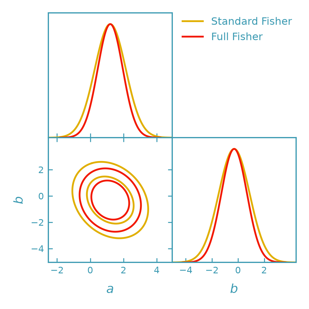
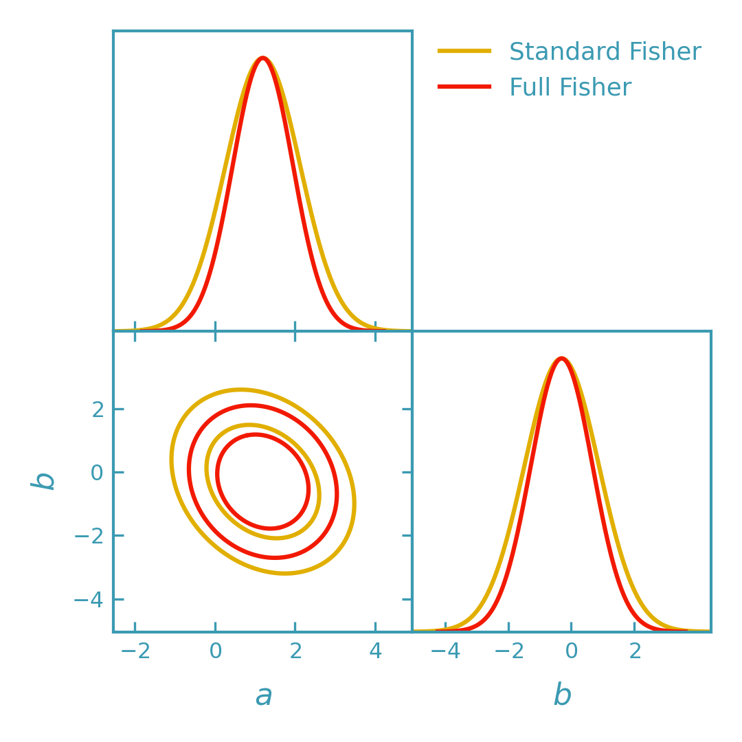
This example compares:

Standard Fisher: uses a fixed covariance \(C(\theta_0)\) and computes \(F = J^\mathsf{T} C^{-1} J\).
Full Gaussian Fisher: allows \(C(\theta)\) and adds the corresponding covariance-derivative terms to the Fisher matrix.
The covariance dependence is chosen to be noticeable but not dominant, while remaining SPD by construction.

>>> import numpy as np
>>> from getdist import plots as getdist_plots
>>> from derivkit.forecast_kit import ForecastKit
>>> from derivkit.forecasting.getdist_fisher_samples import fisher_to_getdist_gaussiannd
>>> # Toy model: data vector in R^3, parameters in R^2
>>> def model(theta):
...     a, b = theta
...     return np.array([a + 0.5 * b, 0.4 * a * b, 0.8 * a + 0.3 * b], dtype=float)
>>> # Parameter-dependent covariance
>>> # C(theta) = C_base + alpha * S(theta) S(theta)^T.
>>> def cov_fn(theta):
...     a, b = theta
...     c_base = np.array(
...         [
...             [0.30, 0.03, 0.01],
...             [0.03, 0.26, 0.02],
...             [0.01, 0.02, 0.22],
...         ],
...         dtype=float,
...     )
...     s = np.array(
...         [
...             [1.0 + 0.9 * a,  0.7 * b,        0.15 * a],
...             [0.25 * b,       0.9 + 0.8 * b,  0.35 * a],
...             [0.10 * a,       0.45 * b,       0.8 + 1.0 * a],
...         ],
...         dtype=float,
...     )
...     alpha = 0.25
...     return c_base + alpha * (s @ s.T)
>>> # Fiducial parameters
>>> theta0 = np.array([1.2, -0.3])
>>> # Build ForecastKit and compute both Fisher matrices
>>> fk = ForecastKit(function=model, theta0=theta0, cov=cov_fn)
>>> fisher_std = fk.fisher()
>>> fisher_full = fk.gaussian_fisher()
>>> # Convert to GetDist GaussianND samples for visualization
>>> gnd_std = fisher_to_getdist_gaussiannd(
...     theta0=theta0,
...     fisher=fisher_std,
...     names=["a", "b"],
...     labels=[r"a", r"b"],
...     label="Standard Fisher",
... )
>>> gnd_full = fisher_to_getdist_gaussiannd(
...     theta0=theta0,
...     fisher=fisher_full,
...     names=["a", "b"],
...     labels=[r"a", r"b"],
...     label="Full Gaussian Fisher",
... )
>>> (gnd_std is not None) and (gnd_full is not None)
True
>>> # Plot the results
>>> dk_yellow = "#e1af00"
>>> dk_red = "#f21901"
>>> line_width = 1.5
>>> plotter = getdist_plots.get_subplot_plotter(width_inch=3.6)
>>> plotter.settings.linewidth_contour = line_width
>>> plotter.settings.linewidth = line_width
>>> plotter.settings.figure_legend_frame = False
>>> plotter.triangle_plot(
...     [gnd_std, gnd_full],
...     params=["a", "b"],
...     legend_labels=["Standard Fisher", "Full Fisher"],
...     legend_ncol=1,
...     filled=[False, False],
...     contour_colors=[dk_yellow, dk_red],
...     contour_lws=[line_width, line_width],
...     contour_ls=["-", "-"],
... )

(png)

Notes#

ForecastKit.fisher() uses a fixed covariance \(C(\theta_0)\) and computes only the mean-derivative term.
ForecastKit.gaussian_fisher() includes the additional covariance-derivative contribution when a parameter-dependent covariance \(C(\theta)\) is provided.