ForecastKit

ForecastKit provides derivative-based tools for local likelihood and posterior analysis. It uses numerical derivatives to construct controlled approximations to a model’s likelihood or posterior around a chosen expansion point.

The toolkit includes multiple Fisher-matrix formalisms, Fisher bias, Laplace approximations, and higher-order DALI expansions. It also provides utilities for contour visualization and posterior sampling based on these local approximations.

All methods rely on DerivativeKit for numerical differentiation and work with arbitrary user-defined models.

Runnable examples illustrating these methods are collected in Examples.

Fisher Information Matrix

The Fisher matrix [1] quantifies how precisely model parameters can be determined from a set of observables under a local Gaussian approximation.

Given:

• parameters \(\theta = (\theta_1, \theta_2, \ldots)\)

• a model mapping parameters to observables \(\nu(\theta)\)

• a data covariance matrix \(C\)

ForecastKit computes the Jacobian

\[J_{i a} = \frac{\partial \nu_i}{\partial \theta_a},\]

using DerivativeKit and CalculusKit, and constructs the standard Fisher matrix

\[F = J^\top C^{-1} J.\]

The Fisher matrix can be inverted to yield the Cramér–Rao lower bound [2] on the parameter covariance matrix under the assumption that the likelihood is locally Gaussian near its maximum. In this approximation, the inverse Fisher matrix provides a lower bound on the achievable variances of unbiased parameter estimators, independent of the specific inference algorithm used. As a result, Fisher matrix methods offer a fast and computationally efficient way to forecast expected parameter constraints without performing full likelihood sampling.

Interpretation

The Fisher matrix provides a fast, local forecast of expected parameter constraints under a Gaussian likelihood approximation.

Examples

The following examples illustrate typical Fisher-forecast workflows:

• A basic Fisher matrix computation: Fisher matrix

• Visualization of Fisher constraints using GetDist: Fisher contours

Generalized Gaussian Fisher

When the data covariance depends on the model parameters, the standard Fisher matrix must be generalized to include derivatives of both the mean and the covariance [3].

For a Gaussian likelihood with mean \(\mu(\theta) = \langle d \rangle\) and covariance \(C(\theta) = \langle (d - \mu)(d - \mu)^{\mathrm T} \rangle\), the Fisher matrix is

\[F_{\alpha\beta} = \frac{1}{2} \mathrm{Tr} \!\left[ C^{-1} C_{,\alpha} C^{-1} C_{,\beta} \right] + \mu_{,\alpha}^{\mathrm T} C^{-1} \mu_{,\beta}.\]

Here \(C_{,\alpha} \equiv \partial C / \partial \theta_\alpha\) and \(\mu_{,\alpha} \equiv \partial \mu / \partial \theta_\alpha\).

This expression reduces to the standard Fisher matrix when the covariance is independent of the parameters.

Interpretation

The generalized Gaussian Fisher provides a consistent local approximation when both the signal and noise depend on the model parameters.

Examples

A worked example is provided in Gaussian Fisher matrix.

X–Y Fisher Formalism

The X–Y Fisher formalism [4] applies when the observables are naturally split into measured inputs \(X\) and outputs \(Y\), both of which are noisy and possibly correlated.

The joint data covariance is written in block form as

\[\begin{split}C = \begin{pmatrix} C_{XX} & C_{XY} \\ C_{XY}^{\mathrm T} & C_{YY} \end{pmatrix},\end{split}\]

and the model predicts the expectation value of the outputs as \(\mu(X, \theta)\).

Assuming the model can be linearized in the latent true inputs \(x\),

\[\mu(x) \simeq \mu(X) + T(X)\,(x - X), \qquad T_{ij} \equiv \frac{\partial \mu_i}{\partial x_j}\Big|_{x=X},\]

the latent variables can be marginalized analytically.

The resulting likelihood for \(Y\) is Gaussian with an effective covariance

\[R = C_{YY} - C_{XY}^{\mathrm T} T^{\mathrm T} - T C_{XY} + T C_{XX} T^{\mathrm T}.\]

The Fisher matrix then takes the same form as the generalized Gaussian Fisher, with the replacement \(C \rightarrow R\):

\[F_{\alpha\beta} = \frac{1}{2} \mathrm{Tr} \!\left[ R^{-1} R_{,\alpha} R^{-1} R_{,\beta} \right] + \mu_{,\alpha}^{\mathrm T} R^{-1} \mu_{,\beta}.\]

Interpretation

The X–Y Fisher matrix consistently propagates uncertainty in the measured inputs into the output covariance, enabling Fisher forecasts when both inputs and outputs are noisy.

Examples

A worked example is provided in X–Y Gaussian Fisher matrix.

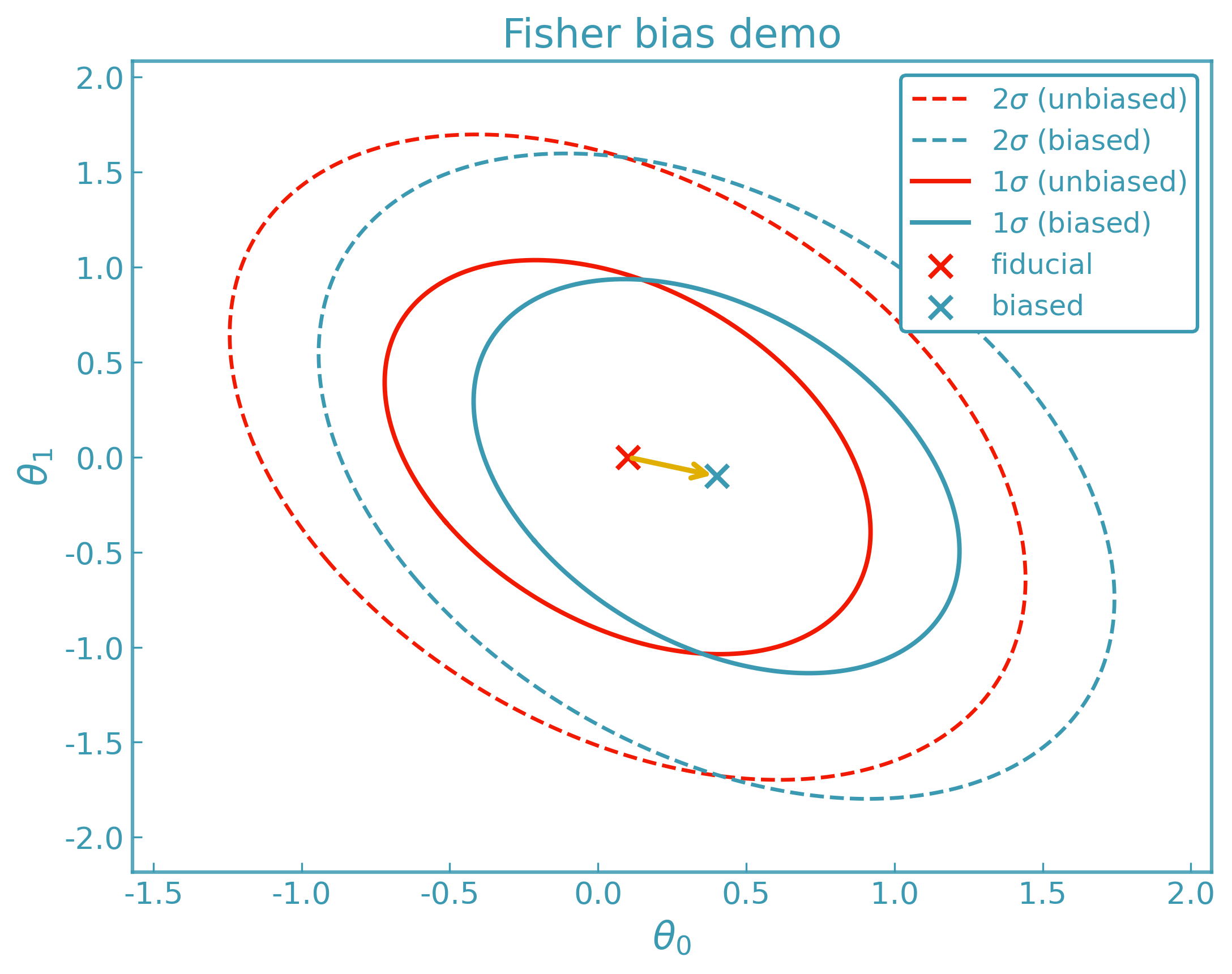
Fisher Bias

Small systematic deviations in the observables can bias inferred parameters [9]. These deviations are encoded as a difference data vector

\[\Delta \nu_i = \nu^{\mathrm{biased}}_i - \nu^{\mathrm{unbiased}}_i.\]

ForecastKit computes the first-order Fisher bias vector

\[b_a = \sum_{i,j} J_{i a}\, C^{-1}_{i j}\, \Delta \nu_j,\]

and the resulting parameter shift

\[\Delta \theta_a = \sum_b (F^{-1})_{a b}\, b_b.\]

ForecastKit returns:

• the bias vector

• the induced parameter shift

• optional visualization of the bias relative to Fisher contours

Interpretation

Fisher bias characterizes the impact of model incompleteness rather than explicit parameter perturbations. The difference vector \(\Delta\nu\) represents a systematic mismatch between the true data-generating model and the model assumed in analysis, evaluated at the same fiducial parameters. The resulting shift \(\Delta\theta\) estimates how the inferred best-fit parameters would move in order to absorb this mismatch if the systematic were neglected. Fisher bias should therefore be interpreted as a diagnostic of whether a given systematic can be safely ignored within a local Gaussian approximation.

In practice, the two data vectors entering \(\Delta\nu\) are obtained by evaluating two models at the same fiducial parameters: a baseline model used for inference and a more complete model that includes additional physical or instrumental systematics. Fisher bias then estimates how the inferred parameters would shift if data generated by the more complete model were analyzed using the baseline model alone. In this sense, Fisher bias quantifies the parameter impact of neglecting specific systematic effects, rather than correcting for them.

The difference vector \(\Delta\nu_i\) can be defined with either sign convention, e.g. \(\pm\Delta\nu_i = \nu_i^{\mathrm{biased}} - \nu_i^{\mathrm{unbiased}}\). The chosen convention fixes the interpretation of the resulting parameter shift \(\Delta\theta\): changing the sign of \(\Delta\nu\) simply reverses the direction of the inferred bias and must be interpreted accordingly.

Examples

A worked example is provided in Fisher bias.

Laplace Approximation

The Laplace approximation [8] replaces the posterior distribution near its maximum by a multivariate Gaussian obtained from a second-order Taylor expansion of the negative log-posterior.

Let the log-posterior be

\[\mathcal{L}(\theta) = -\ln p(\theta \mid d) = -\ln \mathcal{L}(d \mid \theta) -\ln p(\theta).\]

Expanding around the maximum a posteriori (MAP) point \(\hat{\theta}\), where \(\nabla \mathcal{L}(\hat{\theta}) = 0\), gives

\[\mathcal{L}(\theta) \simeq \mathcal{L}(\hat{\theta}) + \frac{1}{2} (\theta - \hat{\theta})^{\mathrm T} H (\theta - \hat{\theta}),\]

where the Hessian matrix is

\[H_{ab} \equiv \left. \frac{\partial^2 \mathcal{L}}{\partial \theta_a \partial \theta_b} \right|_{\theta = \hat{\theta}}.\]

Under this approximation, the posterior is Gaussian,

\[p(\theta \mid d) \approx \mathcal{N} \!\left( \hat{\theta}, \, H^{-1} \right),\]

with covariance given by the inverse Hessian of the negative log-posterior.

In the special case of a flat prior and a Gaussian likelihood, the Hessian reduces to the Fisher information matrix, and the Laplace approximation coincides with the Fisher forecast.

Examples

The following examples illustrate the Laplace approximation workflow:

• A basic Laplace approximation of the posterior: Laplace approximation

• Visualization of Laplace-approximated posteriors using GetDist: Laplace contours

Priors

ForecastKit methods can be used either as likelihood approximations or as posterior approximations. The distinction is whether a prior contribution is included.

Given data \(d\), the posterior is

\[\log p(\theta \mid d) = \log p(d \mid \theta) + \log p(\theta) + \mathrm{const}.\]

ForecastKit represents priors as callables that evaluate a log-density (up to an additive constant). Hard exclusions are encoded by returning -np.inf, corresponding to zero probability outside the allowed region of parameter space.

Where Priors Enter

Priors affect different forecasting methods in distinct ways:

• Fisher and generalized Fisher

  Fisher forecasts are Gaussian likelihood approximations by default. A Gaussian prior may be incorporated analytically by adding its precision matrix to the Fisher matrix.

  For a Gaussian prior with covariance \(C_{\mathrm{prior}}\),

  \[F_{\mathrm{post}} = F_{\mathrm{like}} + C_{\mathrm{prior}}^{-1}.\]

  This yields a Gaussian approximation to the posterior and preserves the Fisher formalism.

• Laplace and DALI approximations

  Laplace and DALI operate directly on the log-posterior when a prior is supplied. In this case, the prior contribution is evaluated explicitly alongside the likelihood expansion, and hard bounds may exclude regions of parameter space.

• Sampling and visualization

  Plotting tools such as GetDist do not apply priors implicitly. If samples are drawn from a Fisher, Laplace, or DALI approximation without including a prior term, the resulting contours correspond to the likelihood approximation alone.

  To visualize posterior constraints, the prior must be included explicitly when generating samples.

Prior Construction

ForecastKit provides a unified prior interface via derivkit.forecasting.priors_core.build_prior().

A prior is constructed by combining one or more prior terms, each of which defines a log-density contribution, and optional hard bounds. The resulting callable evaluates

\[\log p(\theta) = \sum_k \log p_k(\theta),\]

returning -np.inf if any term or bound is violated.

Supported prior terms include:

• uniform (hard bounds)

• multivariate Gaussian and diagonal Gaussian

• log-uniform / Jeffreys

• half-normal and half-Cauchy

• log-normal

• Beta distributions

• Gaussian mixture priors

Interpretation

Priors control identifiability and regularization in local forecasts. They can:

• stabilize ill-conditioned Fisher matrices,

• enforce physical parameter support (e.g. positivity),

• encode external information or weakly informative assumptions,

• determine whether a local approximation should be interpreted as a likelihood forecast or a posterior forecast.

Care should be taken to distinguish numerical regularization from genuine prior information when interpreting forecasted parameter constraints.

Examples

Practical examples demonstrating how priors are incorporated are provided in:

• Including priors in Fisher contours for Fisher forecasts

• Including priors in DALI contours for DALI-based posterior sampling

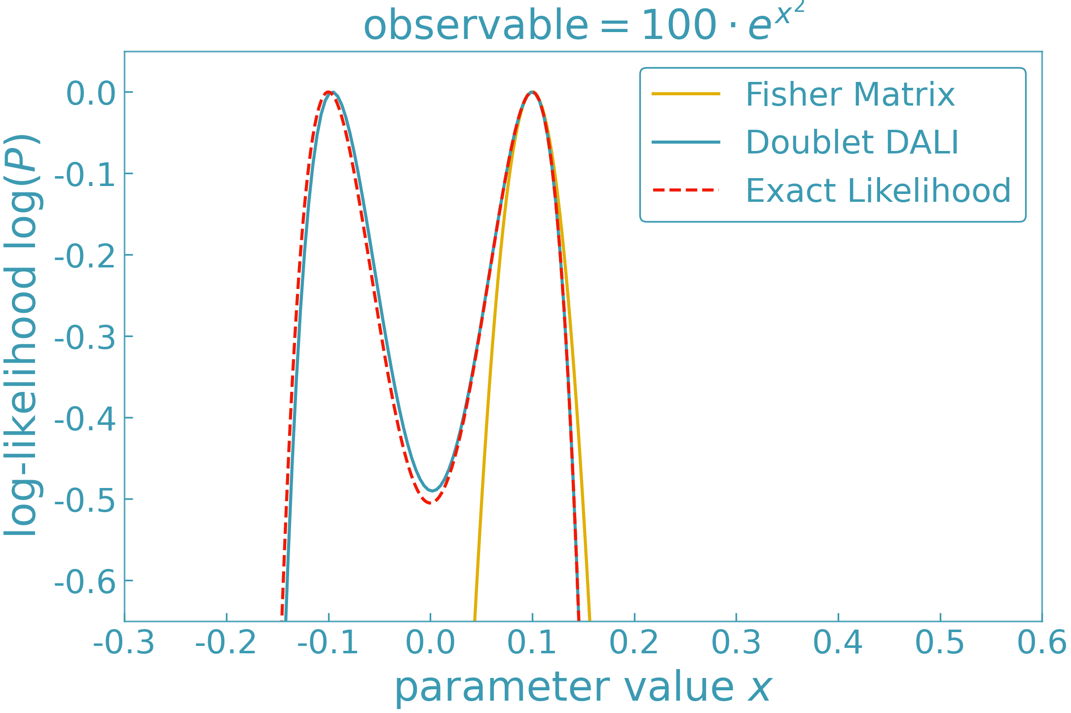
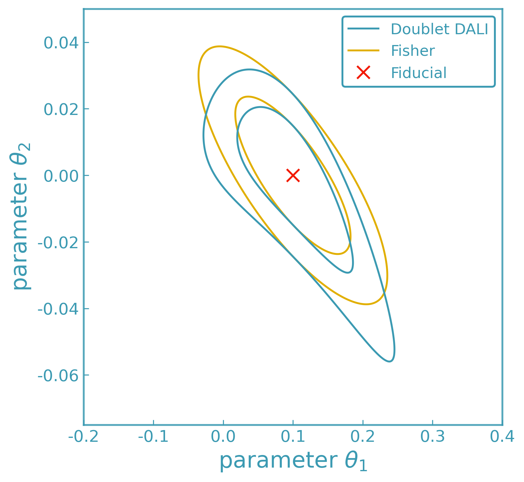
DALI (Higher-Order Forecasting)

The DALI expansion (Derivative Approximation for LIkelihoods; [5]) extends Fisher and Laplace approximations by retaining higher-order derivatives of the likelihood around a chosen expansion point.

Expanding the log-posterior locally in parameter displacements \(\Delta\theta = \theta - \hat{\theta}\), DALI approximates the posterior as

\[\log p(\theta \mid d) \simeq \log p(\hat{\theta} \mid d) - \frac{1}{2} F_{\alpha\beta}\, \Delta\theta_\alpha \Delta\theta_\beta - \frac{1}{3!} D^{(1)}_{\alpha\beta\gamma}\, \Delta\theta_\alpha \Delta\theta_\beta \Delta\theta_\gamma - \frac{1}{4!} D^{(2)}_{\alpha\beta\gamma\delta}\, \Delta\theta_\alpha \Delta\theta_\beta \Delta\theta_\gamma \Delta\theta_\delta + \cdots,\]

where

• \(F_{\alpha\beta}\) is the Fisher matrix,

• \(D^{(1)}_{\alpha\beta\gamma}\) and \(D^{(2)}_{\alpha\beta\gamma\delta}\) are the second-order (doublet) DALI correction terms,

• \(T^{(1)}_{\alpha\beta\gamma\delta}\), \(T^{(2)}_{\alpha\beta\gamma\delta\epsilon}\), and \(T^{(3)}_{\alpha\beta\gamma\delta\epsilon\zeta}\) denote third-order (triplet) DALI correction terms,

all evaluated at the expansion point \(\hat{\theta}\).

For Gaussian data models with parameter-independent covariance, these tensors can be expressed directly in terms of derivatives of the model predictions, allowing DALI to be constructed using numerical derivatives alone.

At second order (“doublet DALI”), the posterior takes the form

\[p(\theta \mid d) \propto \exp\!\Bigg[ -\frac{1}{2} F_{\alpha\beta}\, \Delta\theta_\alpha \Delta\theta_\beta -\frac{1}{2} D^{(1)}_{\alpha\beta\gamma}\, \Delta\theta_\alpha \Delta\theta_\beta \Delta\theta_\gamma +\frac{1}{8} D^{(2)}_{\alpha\beta\gamma\delta}\, \Delta\theta_\alpha \Delta\theta_\beta \Delta\theta_\gamma \Delta\theta_\delta \Bigg].\]

Including third-order (“triplet DALI”) terms introduces additional correction tensors \(T^{(i)}\), which capture higher-order non-Gaussian structure while preserving positive definiteness of the approximation.

Keep in mind that:

• DALI is a local approximation around theta0 and may degrade far from the expansion point.

• DALI may perform poorly for models with weak or sublinear parameter dependence, or when increasing the expansion order does not improve convergence (see discussion in e.g. [5] and section VI.B of arXiv:2211.06534).

• If DALI does not stabilize as the expansion order is increased, numerical posterior sampling (e.g. emcee) should be used to validate the approximation.

Interpretation

DALI provides a controlled hierarchy of local posterior approximations, reducing to the Fisher and Laplace limits when higher-order derivatives vanish.

Examples

The following examples illustrate the DALI approximation workflow:

• A basic DALI expansion of the posterior: DALI tensors

• Visualization of DALI-expanded posteriors using GetDist: DALI contours

Posterior Sampling and Visualization

ForecastKit provides utilities to draw samples directly from Fisher, Laplace, or DALI-expanded posteriors and to convert them into GetDist-compatible [6] MCSamples objects.

This enables:

• posterior sampling based on local likelihood approximations using emcee [7]

• easy integration with GetDist for contour plotting and statistical summaries

• direct contour visualization and uncertainty propagation

• comparison between Fisher, Laplace, and DALI forecasts

These workflows are designed for forecasting and local posterior analysis, providing fast and controlled approximations to parameter constraints without requiring full likelihood evaluations with MCMC or nested sampling methods.

Examples:

Worked examples are provided in: - Fisher contours for Fisher-based GetDist samples - DALI contours for DALI-based posterior sampling - Laplace contours for Laplace approximations

Backend Notes

• If method is omitted, the adaptive derivative backend is used.

• Any DerivativeKit backend may be selected (finite differences, Ridders, Gauss–Richardson, polynomial fits, etc.).

• Changing the derivative backend affects only how derivatives are computed, not the forecasting logic itself.

ForecastKit is fully modular and designed to scale from simple Gaussian forecasts to higher-order likelihood expansions with minimal code changes.

References

[1]

Wikipedia, Fisher information matrix, https://en.wikipedia.org/wiki/Fisher_information

[2]

Wikipedia, Cramér–Rao bound, https://en.wikipedia.org/wiki/Cramér–Rao_bound

[3]

M. Tegmark et al., Karhunen-Loeve eigenvalue problems in cosmology: how should we tackle large data sets?, https://arxiv.org/abs/1404.2854

[4]

A. Heavens et al., Generalised Fisher Matrices, https://arxiv.org/abs/1404.2854

[5] (1,2)

E. Sellentin et al., Breaking the spell of Gaussianity: forecasting with higher order Fisher matrices https://arxiv.org/abs/1401.6892

[6]

A. Lewis, GetDist: a Python package for analysing Monte Carlo samples, https://arxiv.org/abs/1910.13970

[7]

D. Foreman-Mackey et al., emcee: The MCMC Hammer, https://arxiv.org/abs/1202.3665

[8]

Wikipedia, Laplace’s approximation, https://en.wikipedia.org/wiki/Laplace%27s_approximation

[9]

A. Amara and A. Réfrégier, Systematic Bias in Cosmic Shear: Beyond the Fisher Matrix, https://arxiv.org/abs/0710.5171