 DerivativeKit#
DerivKit implements several complementary derivative engines. Each has different strengths depending on smoothness, noise level, and computational cost.
This page gives an overview of the main methods featured in DerivativeKit,
how they work, and when to use each one.
All methods are accessed through the same DerivativeKit interface and can be swapped without changing downstream code.
Runnable examples illustrating these methods are collected in Examples.
Finite Differences#
How it works:
Estimate derivatives by evaluating the function at points around x0 and
combining them into a central-difference stencil [1].
In general, a central finite-difference approximation to the first derivative
can be written as a weighted sum over function evaluations at symmetric offsets
around x0:
where h is the step size (the spacing between adjacent stencil points),
and the stencil coefficients c_k satisfy symmetry conditions
(c_{-k} = -c_k) and are chosen to cancel low-order truncation errors.
The integer m determines the stencil width (e.g. m=1 for a 3-point
stencil, m=2 for a 5-point stencil). The coefficients c_k are computed
using standard algorithms (such as Fornberg’s method), which construct
finite-difference weights by enforcing the desired order of accuracy for a given stencil.
Higher-order stencils improve accuracy by cancelling additional error terms, at the cost of more function evaluations.
DerivKit implementation:
3, 5, 7, 9-point central stencils
Richardson extrapolation [4] (reduces truncation error)
Ridders extrapolation [5] (adaptive error control)
Gauss–Richardson extrapolation (GRE) [3] (noise-robust variant)
Use when:
The function is smooth and cheap to evaluate
Noise is low or absent
You want fast derivatives with minimal overhead
Avoid when:
The function is noisy or discontinuous
Step-size tuning is difficult or unstable
Function evaluations are expensive
Examples:
A basic finite-difference example is shown in Finite differences.
Simple Polynomial Fit#
How it works:
Sample points in a small, user-controlled window around x0 and fit a
fixed-order polynomial (e.g. quadratic or cubic) on a simple grid. The
derivative at x0 is taken from the analytic derivative of the fitted polynomial
[2].
The expression for a first derivative from a centered quadratic fit
is:
where a_1 is the fitted linear coefficient of the polynomial.
DerivKit implementation:
User-chosen window and polynomial degree
Low overhead and transparent behaviour
Includes diagnostics on fit quality and conditioning
Use when:
The function is smooth but mildly noisy
You want a simple, local smoothing method
A fixed window and polynomial degree are sufficient
Avoid when:
Noise is strong or highly irregular
The fit becomes ill-conditioned in the chosen window
Examples:
A basic polyfit example is shown in Local polynomial fit.
Adaptive Polynomial Fit#
How it works:
Build a Chebyshev-spaced grid around x0, rescale offsets to a stable interval,
and fit a local polynomial with optional ridge regularisation.
The method can enlarge the grid if there are too few samples
and adjust the effective polynomial degree.
It also reports detailed diagnostics on fit quality and suggests improvements
if the derivative appears unreliable.
[2].
For a centered polynomial fit of degree d,
the first derivative is
and in particular
where a_k are the fitted polynomial coefficients.
Sampling strategy:
Default: symmetric Chebyshev nodes around
x0with automatic half-width (viaspacing="auto"andbase_abs)Domain-aware: interval is clipped to stay inside a given
(lo, hi)domainCustom grids: user can supply explicit offsets or absolute sample locations
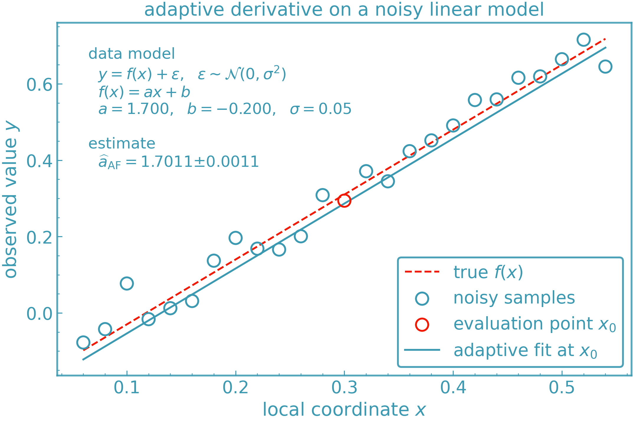
Below is a visual example of the derivkit.adaptive_fit module estimating
the first derivative of a nonlinear function in the presence of noise. The method
selectively discards outlier points before fitting a polynomial, resulting in a
robust and smooth estimate.
DerivKit implementation:
Scales offsets before fitting to reduce conditioning
Optional ridge term to stabilise ill-conditioned Vandermonde systems
Checks fit quality and flags “obviously bad” derivatives with suggestions for improvement
Optional diagnostics dictionary with sampled points, fit metrics, and metadata
Use when:
The function is noisy, irregular, or numerically delicate
Finite differences or simple polyfits fail
You want diagnostics to understand derivative quality
Avoid when:
The function is extremely smooth and cheap to evaluate
Minimal overhead is a priority
You want a minimal-overhead solution for very smooth functions
Examples:
A basic adaptive polyfit example is shown in Adaptive polynomial fit.
Tabulated Functions#
How it works:
When the target function is provided as tabulated data (x, y), DerivKit first
wraps the table in a lightweight interpolator and then applies any of the
available derivative engines to the interpolated function.
Internally, tabulated data are represented by
derivkit.tabulated_model.one_d.Tabulated1DModel, which exposes a callable
interface compatible with all derivative methods.
DerivKit implementation:
Supports scalar-, vector-, and tensor-valued tabulated outputs
Uses fast linear interpolation via
numpy.interpSeamlessly integrates with finite differences, adaptive fit, local polynomial, and Fornberg methods
Identical API to function-based differentiation via
DerivativeKit
Use when:
The function is only available as discrete samples
Evaluating the function on demand is expensive or impossible
You want to reuse DerivKit’s derivative engines on interpolated data
Avoid when:
The tabulation is too coarse to resolve derivatives
The function has sharp features not captured by interpolation
Exact derivatives are required
Examples:
See Tabulated derivatives for a basic example using tabulated data.
JAX Autodiff#
How it works:
JAX provides automatic differentiation for Python functions written using jax.numpy. Instead of estimating derivatives numerically, autodiff propagates derivatives analytically through the computational graph, yielding exact derivatives up to machine precision.
A key distinction from finite differences or local fits is that autodiff stays close to the implemented functional form: it differentiates the same computation used to produce the model outputs, rather than estimating derivatives from nearby perturbed evaluations. When the model is smooth and expressed end-to-end in JAX, the resulting derivative typically has very small numerical error and does not introduce additional differencing noise.
This avoids step-size choices, local sampling, and numerical differencing. This does not mean autodiff is universally superior. Autodiff differentiates the implemented computation. If that computation already contains approximations (splines, table lookups, iterative solvers, discontinuities, clipping, etc.), autodiff returns the exact derivative of that effective function, which may not match the derivative of the intended underlying model.
Its applicability is therefore limited to fully JAX-compatible, analytic models and does not extend to noisy, interpolated, or externally evaluated functions.
DerivKit implementation:
Exposed as an optional reference backend and not registered as a standard
DerivativeKitmethodIntended primarily for sanity checks and validation
Not a core focus of DerivKit, which targets workflows where models are:
noisy
tabulated
interpolated
externally evaluated
incompatible with automatic differentiation
Use when:
The function is analytic and fully JAX-compatible
You want an exact reference derivative for comparison
You are prototyping or testing derivative workflows
Avoid when:
The function is noisy, tabulated, interpolated, or provided by an external numerical software (e.g. Boltzmann solvers or many cosmology emulators that rely on interpolation or precomputed grids rather than end-to-end autodiff)
You need production robustness or broad applicability
JAX compatibility cannot be guaranteed
In most scientific workflows targeted by DerivKit, the adaptive polynomial fit or finite-difference methods above are more appropriate.
Installation details for the JAX module are described in Installation. We do not recommend JAX for production use within DerivKit at this time.