 Laplace contours#
This page shows how to visualize Laplace-approximation posteriors using GetDist,
starting from a Laplace approximation computed with DerivKit.
The focus here is what to do next once you already have a Laplace approximation: how to turn it into confidence contours or samples for quick inspection, comparison, and plotting.
This is intended for fast exploration and visualization, not as a replacement for full likelihood-based inference or full MCMC sampling.
If you are looking for:
how the Laplace approximation is defined and interpreted, see ForecastKit
how to compute a Laplace approximation with DerivKit, see Laplace approximation
Two complementary visualization workflows are supported:
conversion of the Laplace Gaussian into an analytic Gaussian for
GetDistMonte Carlo samples drawn from the Laplace Gaussian, returned as
getdist.MCSamples
Both outputs can be passed directly to GetDist plotting utilities (e.g. triangle / corner plots).
Notes and conventions#
The Laplace approximation is a local Gaussian centered on the MAP point
theta_map. In other words, the Laplace mean istheta_mapby construction.The Laplace covariance is the inverse Hessian of the negative log-posterior at
theta_map(up to numerical regularization).getdist.MCSamples.loglikesstores minus the log-posterior (up to an additive constant), following GetDist conventions.For strongly non-Gaussian posteriors or curved degeneracies far from the MAP, consider using DALI or a full sampler instead.
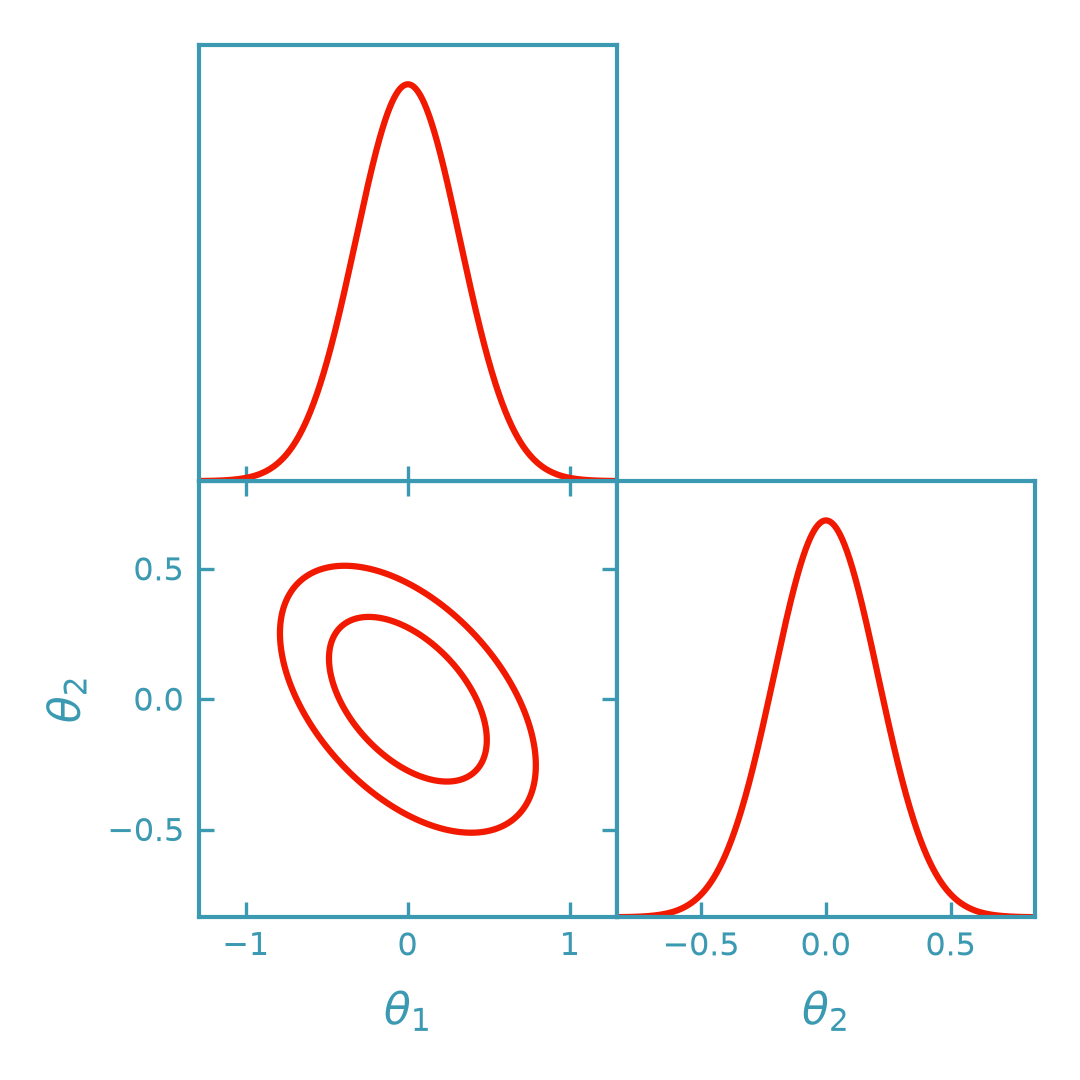
Analytic Gaussian (no sampling)#
Convert the Laplace approximation into an analytic Gaussian object compatible with GetDist, then plot contours using GetDist.
>>> import numpy as np
>>> from getdist import plots as getdist_plots
>>> from derivkit import ForecastKit
>>> # Linear–Gaussian likelihood with Gaussian prior (posterior is exactly Gaussian).
>>> observed_y = np.array([1.2, -0.4], dtype=float)
>>> design_matrix = np.array([[1.0, 0.5], [0.2, 1.3]], dtype=float)
>>>
>>> data_cov = np.array([[0.30**2, 0.0], [0.0, 0.25**2]], dtype=float)
>>> data_prec = np.linalg.inv(data_cov)
>>>
>>> prior_mean = np.array([0.0, 0.0], dtype=float)
>>> prior_cov = np.array([[1.0**2, 0.0], [0.0, 1.5**2]], dtype=float)
>>> prior_prec = np.linalg.inv(prior_cov)
>>> # Define the negative log-posterior
>>> def neg_logposterior(theta):
...     theta = np.asarray(theta, dtype=float)
...     r = observed_y - design_matrix @ theta
...     nll = 0.5 * (r @ data_prec @ r)
...     d = theta - prior_mean
...     nlp = 0.5 * (d @ prior_prec @ d)
...     return float(nll + nlp)
>>> # Initial guess for the MAP point
>>> theta_map0 = np.array([0.0, 0.0], dtype=float)
>>> fk0 = ForecastKit(function=None, theta0=theta_map0, cov=np.eye(2))
>>> out = fk0.laplace_approximation(
...     neg_logposterior=neg_logposterior,
...     theta_map=theta_map0,
...     method="finite",
...     stepsize=1e-3,
...     num_points=5,
...     extrapolation="ridders",
...     levels=4
... )
>>> theta_map = np.asarray(out["theta_map"], dtype=float)
>>> cov = np.asarray(out["cov"], dtype=float)
>>> fisher = np.linalg.pinv(cov)
>>> theta_map.shape == (2,) and cov.shape == (2, 2)
True
>>> # ForecastKit GetDist helper fixes the mean to fk.theta0, so set theta0=theta_map.
>>> fk = ForecastKit(function=None, theta0=theta_map, cov=np.eye(2))
>>> samples = fk.getdist_fisher_gaussian(
...     fisher=fisher,
...     names=["theta1", "theta2"],
...     labels=[r"\theta_1", r"\theta_2"],
...     label="Laplace (Gaussian)",
... )
>>> dk_red = "#f21901"
>>> line_width = 1.5
>>> plotter = getdist_plots.get_subplot_plotter(width_inch=3.6)
>>> plotter.settings.linewidth_contour = line_width
>>> plotter.settings.linewidth = line_width
>>> plotter.triangle_plot(
...     [samples],
...     params=["theta1", "theta2"],
...     filled=[False],
...     contour_colors=[dk_red],
...     contour_lws=[line_width],
...     contour_ls=["-"],
... )
(png)

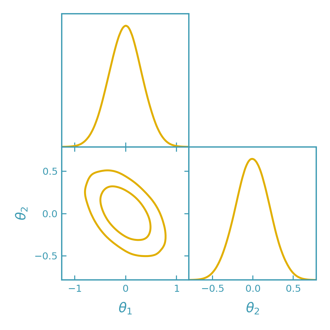
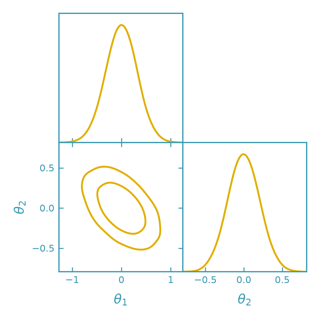
Sampling from the Laplace Gaussian#
For more flexibility (e.g. marginal histograms, bounds, or combining with other samples), draw Monte Carlo samples from the Laplace Gaussian and plot them with GetDist.
>>> import numpy as np
>>> from getdist import plots as getdist_plots
>>> from derivkit import ForecastKit
>>>
>>> observed_y = np.array([1.2, -0.4], dtype=float)
>>> design_matrix = np.array([[1.0, 0.5], [0.2, 1.3]], dtype=float)
>>>
>>> data_cov = np.array([[0.30**2, 0.0], [0.0, 0.25**2]], dtype=float)
>>> data_prec = np.linalg.inv(data_cov)
>>>
>>> prior_mean = np.array([0.0, 0.0], dtype=float)
>>> prior_cov = np.array([[1.0**2, 0.0], [0.0, 1.5**2]], dtype=float)
>>> prior_prec = np.linalg.inv(prior_cov)
>>>
>>> def neg_logposterior(theta):
...     theta = np.asarray(theta, dtype=float)
...     r = observed_y - design_matrix @ theta
...     nll = 0.5 * (r @ data_prec @ r)
...     d = theta - prior_mean
...     nlp = 0.5 * (d @ prior_prec @ d)
...     return float(nll + nlp)
>>>
>>> theta_map0 = np.array([0.0, 0.0], dtype=float)
>>> fk0 = ForecastKit(function=None, theta0=theta_map0, cov=np.eye(2))
>>> out = fk0.laplace_approximation(
...     neg_logposterior=neg_logposterior,
...     theta_map=theta_map0,
...     method="finite",
...     stepsize=1e-3,
...     num_points=5,
...     extrapolation="ridders",
...     levels=4,
... )
>>> theta_map = np.asarray(out["theta_map"], dtype=float)
>>> cov = np.asarray(out["cov"], dtype=float)
>>> fisher = np.linalg.pinv(cov)
>>>
>>> fk = ForecastKit(function=None, theta0=theta_map, cov=np.eye(2))
>>> samples = fk.getdist_fisher_samples(
...     fisher=fisher,
...     names=["theta1", "theta2"],
...     labels=[r"\theta_1", r"\theta_2"],
...     store_loglikes=True,
...     label="Laplace (samples)",
... )
>>>
>>> dk_yellow = "#e1af00"
>>> line_width = 1.5
>>> plotter = getdist_plots.get_subplot_plotter(width_inch=3.6)
>>> plotter.settings.linewidth_contour = line_width
>>> plotter.settings.linewidth = line_width
>>> plotter.triangle_plot(
...     [samples],
...     params=["theta1", "theta2"],
...     filled=False,
...     contour_colors=[dk_yellow],
...     contour_lws=[line_width],
...     contour_ls=["-"],
... )
>>> samples.numrows > 0
True
(png)