 X–Y Gaussian Fisher matrix#
This section shows how to compute a Gaussian Fisher matrix when both the inputs and outputs of a model are noisy and may be correlated.
The X–Y Gaussian Fisher formalism applies when the observables are naturally split into measured inputs \(X\) and outputs \(Y\), each with associated measurement uncertainty. Rather than treating the inputs as exact, their uncertainties are propagated into an effective covariance for the outputs.
For a model predicting the mean output \(\mu_{xy}(x, \theta)\) and a joint input–output covariance
input uncertainty is incorporated through a local linearization of the model with respect to the inputs. This yields an effective output covariance \(R(\theta)\), which replaces \(C_{yy}\) in the Gaussian likelihood and Fisher matrix.
The primary interface for this workflow is
derivkit.forecasting.fisher_xy.build_xy_gaussian_fisher_matrix().
For conceptual background and interpretation, see ForecastKit.
The X–Y Gaussian Fisher is useful when measurement uncertainty in the inputs cannot be neglected and must be consistently propagated into parameter constraints.
A mock example#
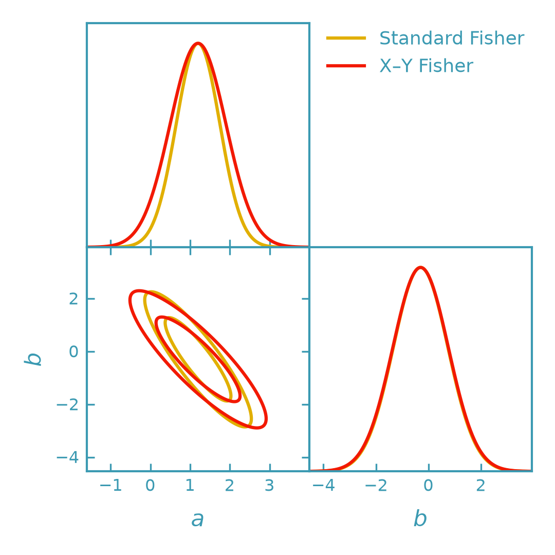
This example compares:
Standard Fisher: treats the measured inputs \(x_0\) as exact and uses only the output covariance \(C_{yy}\).
X–Y Fisher: propagates input uncertainty using \(C_{xx}\) and \(C_{xy}\), leading to a Fisher matrix defined in terms of the effective covariance \(R(\theta)\).
>>> import numpy as np
>>> from getdist import plots as getdist_plots
>>> from derivkit import ForecastKit
>>> # Toy model: x in R^2, theta in R^2, y in R^3
>>> def mu_xy(x, theta):
...     x = np.asarray(x, dtype=float)
...     theta = np.asarray(theta, dtype=float)
...     a, b = theta
...     x0, x1 = x
...     return np.array(
...         [
...             a * x0 + 0.6 * b,
...             a * (x1 ** 2) + 0.3 * b,
...             a * (x0 + 0.5 * x1) + b * x0,
...         ],
...         dtype=float,
...     )
>>> # Fiducial parameters and inputs
>>> theta0 = np.array([1.2, -0.3])
>>> x0 = np.array([0.7, 1.1])
>>> # Covariance blocks
>>> cyy = np.array(
...     [
...         [0.25, 0.04, 0.01],
...         [0.04, 0.20, 0.03],
...         [0.01, 0.03, 0.18],
...     ],
...     dtype=float,
... )
>>> cxx = np.array([[0.06, 0.02], [0.02, 0.10]], dtype=float)
>>> cxy = np.array(
...     [
...         [0.03, -0.01, 0.02],
...         [0.00,  0.02, -0.015],
...     ],
...     dtype=float,
... )
>>> # Build stacked covariance for [x, y]
>>> top = np.hstack([cxx, cxy])
>>> bot = np.hstack([cxy.T, cyy])
>>> cov_xy = np.vstack([top, bot])
>>> # Standard Fisher: treat x0 as exact and use only Cyy
>>> def mu_theta(theta):
...     return mu_xy(x0, theta)
>>> fk_std = ForecastKit(function=mu_theta, theta0=theta0, cov=cyy)
>>> fisher_std = fk_std.fisher()
>>> # X–Y Fisher: propagate input uncertainty from the stacked covariance
>>> fk_xy = ForecastKit(function=None, theta0=theta0, cov=cyy)
>>> fisher_xy = fk_xy.xy_fisher(
...     x0=x0,
...     mu_xy=mu_xy,
...     cov_xy=cov_xy,
... )
>>> # Convert to GetDist GaussianND objects for visualization (via ForecastKit)
>>> gnd_std = fk_std.getdist_fisher_gaussian(
...     fisher=fisher_std,
...     names=["a", "b"],
...     labels=[r"a", r"b"],
...     label="Standard Fisher",
... )
>>> gnd_xy = fk_xy.getdist_fisher_gaussian(
...     fisher=fisher_xy,
...     names=["a", "b"],
...     labels=[r"a", r"b"],
...     label="X–Y Fisher",
... )
>>> (gnd_std is not None) and (gnd_xy is not None)
True
>>> # Plot the contours
>>> dk_yellow = "#e1af00"
>>> dk_red = "#f21901"
>>> line_width = 1.5
>>> plotter = getdist_plots.get_subplot_plotter(width_inch=3.6)
>>> plotter.settings.linewidth_contour = line_width
>>> plotter.settings.linewidth = line_width
>>> plotter.settings.figure_legend_frame = False
>>> plotter.triangle_plot(
...     [gnd_std, gnd_xy],
...     params=["a", "b"],
...     legend_labels=["Standard Fisher", "X–Y Fisher"],
...     legend_ncol=1,
...     filled=[False, False],
...     contour_colors=[dk_yellow, dk_red],
...     contour_lws=[line_width, line_width],
...     contour_ls=["-", "-"],
...     )
(png)

Notes#
The standard Fisher treats the measured inputs \(x_0\) as exact and uses the output covariance \(C_{yy}\) directly.
The X–Y Fisher propagates input uncertainty using the input and cross covariances \(C_{xx}\) and \(C_{xy}\) through an effective covariance \(R(\theta)\), constructed from the local sensitivity matrix \(T = \frac{\mathrm{d}\mu_{xy}(x,\theta)}{\mathrm{d}x}\bigg|_{(x_0,\theta)}\) evaluated at \((x_0, \theta)\).
The resulting Fisher matrix depends on the derivative backend used to compute \(T\). The choice of method and derivative settings is controlled via
methodand**dk_kwargs.