Fisher contours#

This page shows how to visualize Fisher-matrix forecasts using GetDist, starting from a Fisher matrix computed with derivkit.forecast_kit.ForecastKit.

The focus here is what to do next once you already have a Fisher matrix: how to turn it into confidence contours or samples for quick inspection, comparison, and plotting.

If you are looking for:

how the Fisher matrix is defined and interpreted, see ForecastKit
how to compute a Fisher matrix with DerivKit, see Fisher matrix

Two complementary visualization workflows are supported:

passing an analytic Fisher Gaussian to GetDist, which handles sampling internally for visualization
explicitly drawing samples from the Fisher Gaussian and returning them as getdist.MCSamples

Both outputs can be passed directly to GetDist plotting utilities (e.g. triangle / corner plots).

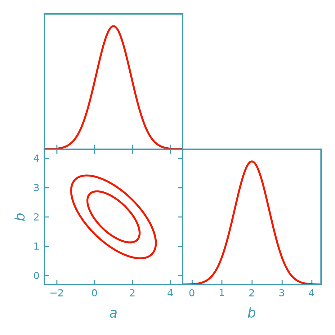
Analytic Gaussian#

Convert the Fisher matrix into an analytic Gaussian object compatible with GetDist. The Gaussian distribution is passed directly to GetDist for visualization, without explicitly drawing samples in DerivKit.

>>> import numpy as np
>>> from getdist import plots as getdist_plots
>>> from derivkit import ForecastKit
>>> # Define a simple toy model
>>> def model(theta):
...     a, b = theta
...     return np.array([a, b, a + 2.0 * b], dtype=float)
>>> # Fiducial parameters and covariance
>>> theta0 = np.array([1.0, 2.0])
>>> cov = np.eye(3)
>>> # Compute Fisher matrix
>>> fk = ForecastKit(function=model, theta0=theta0, cov=cov)
>>> fisher = fk.fisher(
...     method="finite",
...     stepsize=1e-2,
...     num_points=5,
...     extrapolation="ridders",
...     levels=4,
... )
>>> # Construct a Gaussian object for GetDist-managed sampling and visualization
>>> gnd = fk.getdist_fisher_gaussian(
...     fisher=fisher,
...     names=["a", "b"],
...     labels=[r"a", r"b"],
...     label="Fisher (Gaussian)",
... )
>>> # Plot Fisher ellipses in DerivKit red (rendered by the docs build)
>>> dk_red = "#f21901"
>>> line_width = 1.5
>>> plotter = getdist_plots.get_subplot_plotter(width_inch=3.6)
>>> plotter.settings.linewidth_contour = line_width
>>> plotter.settings.linewidth = line_width
>>> plotter.triangle_plot(
...     [gnd],
...     params=["a", "b"],
...     filled=[False],
...     contour_colors=[dk_red],
...     contour_lws=[line_width],
...     contour_ls=["-"],
... )
>>> isinstance(gnd, object)
True

(png)

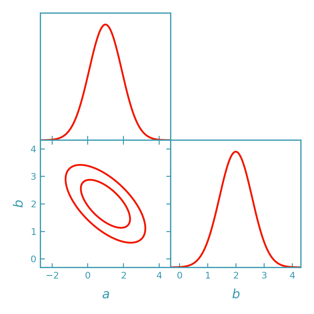
Sampling from the Fisher Gaussian#

Alternatively, explicitly draw Monte Carlo samples from the Fisher Gaussian and return them as a getdist.MCSamples object. This provides direct access to the samples for further analysis, applying bounds, or combining with other samples.

>>> import numpy as np
>>> from getdist import plots as getdist_plots
>>> from derivkit import ForecastKit
>>> # Define a simple toy model
>>> def model(theta):
...     a, b = theta
...     return np.array([a, b, a + 2.0 * b], dtype=float)
>>> # Fiducial parameters and covariance
>>> theta0 = np.array([1.0, 2.0])
>>> cov = np.eye(3)
>>> # Compute Fisher matrix
>>> fk = ForecastKit(function=model, theta0=theta0, cov=cov)
>>> fisher = fk.fisher(
...     method="finite",
...     stepsize=1e-2,
...     num_points=5,
...     extrapolation="ridders",
...     levels=4,
... )
>>> # Draw samples from the Fisher Gaussian
>>> samples = fk.getdist_fisher_samples(
...     fisher=fisher,
...     names=["a", "b"],
...     labels=[r"a", r"b"],
...     store_loglikes=True,
...     label="Fisher (samples)",
... )
>>> # Plot sample-based contours in DerivKit red (rendered by the docs build)
>>> dk_red = "#f21901"
>>> line_width = 1.5
>>> plotter = getdist_plots.get_subplot_plotter(width_inch=3.6)
>>> plotter.settings.linewidth_contour = line_width
>>> plotter.settings.linewidth = line_width
>>> plotter.triangle_plot(
...     [samples],
...     params=["a", "b"],
...     filled=False,
...     contour_colors=[dk_red],
...     contour_lws=[line_width],
...     contour_ls=["-"],
... )
>>> samples.numrows > 0
True

(png)

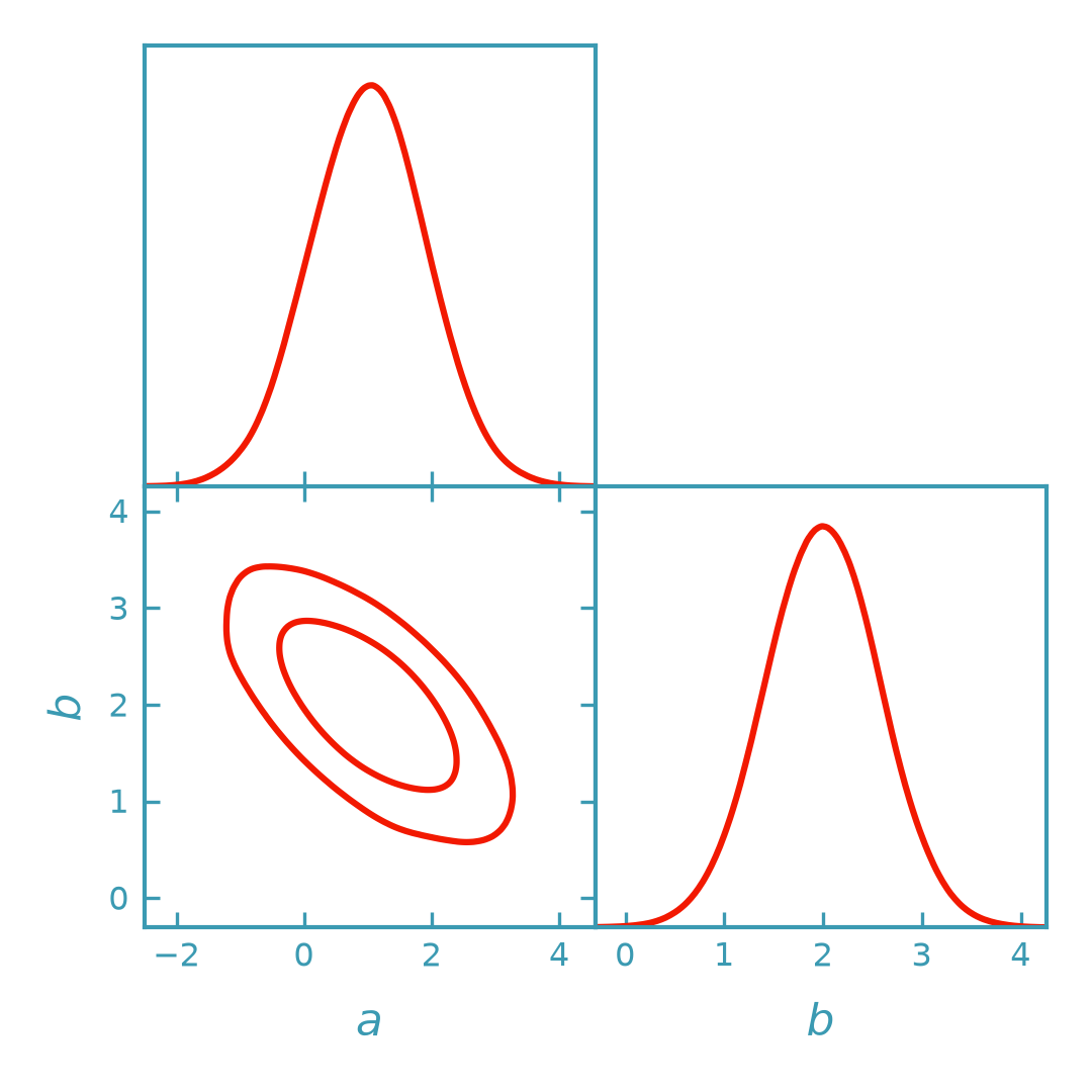
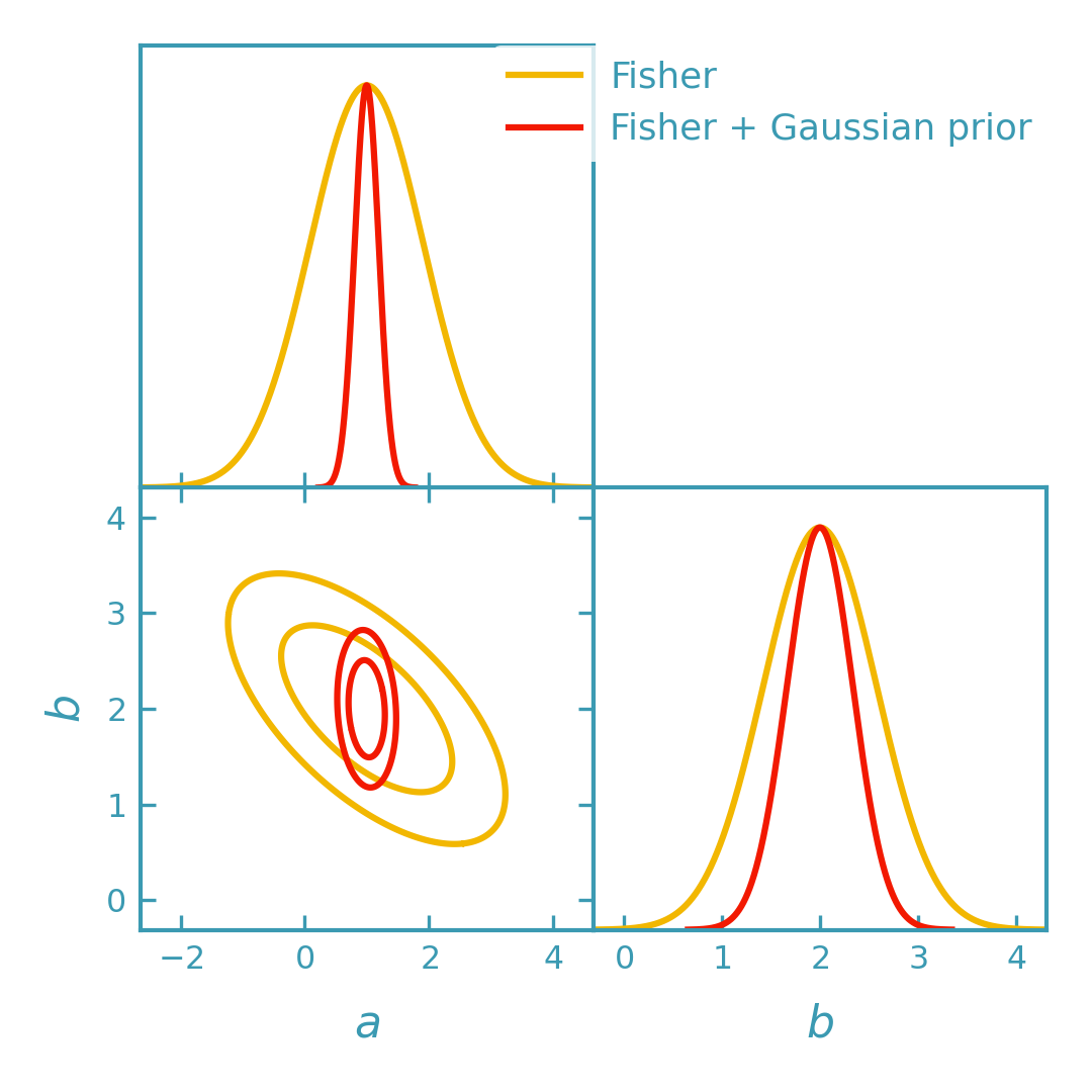
Including Gaussian priors in Fisher forecast#

Gaussian priors can be included by adding their precision matrix (the inverse prior covariance) to the Fisher matrix before converting to GetDist objects. Below we overlay the original Fisher contours (red) with the Fisher+prior contours (yellow).

>>> import numpy as np
>>> from getdist import plots as getdist_plots
>>> from derivkit import ForecastKit
>>> np.set_printoptions(precision=8, suppress=True)
>>> # Same toy model as above
>>> def model(theta):
...     a, b = theta
...     return np.array([a, b, a + 2.0 * b], dtype=float)
>>> theta0 = np.array([1.0, 2.0])
>>> cov = np.eye(3)
>>> # Fisher from the example above
>>> fk = ForecastKit(function=model, theta0=theta0, cov=cov)
>>> fisher_like = fk.fisher()
>>> # Gaussian prior: sigma_a = 0.6, sigma_b = 0.8 (diagonal prior covariance)
>>> sigma_prior = np.array([0.6, 0.8], dtype=float)
>>> fisher_prior = np.diag(1.0 / sigma_prior**2)
>>> fisher_post = fisher_like + fisher_prior
>>> # Convert both to analytic GetDist Gaussians
>>> g_like = fk.getdist_fisher_gaussian(
...     fisher=fisher_like,
...     names=["a", "b"],
...     labels=[r"a", r"b"],
...     label="Fisher",
... )
>>> g_post = fk.getdist_fisher_gaussian(
...     fisher=fisher_post,
...     names=["a", "b"],
...     labels=[r"a", r"b"],
...     label="Fisher + Gaussian prior",
... )
>>> # Overlay contours: red (likelihoods-only) and yellow (with prior)
>>> dk_red = "#f21901"
>>> dk_yellow = "#f2b701"
>>> line_width = 1.5
>>> plotter = getdist_plots.get_subplot_plotter(width_inch=3.6)
>>> plotter.settings.linewidth_contour = line_width
>>> plotter.settings.linewidth = line_width
>>> plotter.settings.figure_legend_frame = False
>>> plotter.settings.legend_rect_border = False
>>> plotter.triangle_plot(
...     [g_like, g_post],
...     params=["a", "b"],
...     filled=[False, False],
...     contour_colors=[dk_red, dk_yellow],
...     contour_lws=[line_width, line_width],
...     contour_ls=["-", "-"],
... )
>>> (g_like is not None) and (g_post is not None)
True

(png)

Including correlated Gaussian priors#

A correlated Gaussian prior can be included by adding its precision matrix to the Fisher matrix. Unlike a diagonal prior, a correlated prior contains off-diagonal covariance terms and can therefore change the orientation of the resulting confidence contours.

Below, the Fisher-only contours (red) are compared with those obtained after including a correlated Gaussian prior (yellow).

The derivkit.forecasting.priors_core.prior_gaussian() utility constructs the corresponding log-prior, while its covariance is used directly to update the Fisher matrix. The prior mean is set to the fiducial point theta0, so the posterior Gaussian remains centered there.

>>> import numpy as np
>>> from getdist import plots as getdist_plots
>>> from derivkit import ForecastKit
>>> from derivkit.forecasting.priors_core import prior_gaussian
>>> def model(theta):
...     a, b = theta
...     return np.array([a, b, a + 2.0 * b], dtype=float)
>>> theta0 = np.array([1.0, 2.0])
>>> fk = ForecastKit(function=model, theta0=theta0, cov=np.eye(3))
>>> fisher_like = fk.fisher()
>>> sigma_a, sigma_b, rho = 0.6, 0.8, -0.7
>>> cov_prior = np.array([
...     [sigma_a**2, rho * sigma_a * sigma_b],
...     [rho * sigma_a * sigma_b, sigma_b**2],
... ])
>>> logprior = prior_gaussian(mean=theta0, cov=cov_prior)
>>> fisher_post = fisher_like + np.linalg.inv(cov_prior)
>>> g_like = fk.getdist_fisher_gaussian(
...     fisher=fisher_like, names=["a", "b"], labels=[r"a", r"b"],
...     label="Fisher",
... )
>>> g_post = fk.getdist_fisher_gaussian(
...     fisher=fisher_post, names=["a", "b"], labels=[r"a", r"b"],
...     label="Fisher + correlated prior",
... )
>>> dk_red = "#f21901"
>>> dk_yellow = "#f2b701"
>>> line_width = 1.5
>>> plotter = getdist_plots.get_subplot_plotter(width_inch=3.6)
>>> plotter.settings.linewidth_contour = line_width
>>> plotter.settings.linewidth = line_width
>>> plotter.triangle_plot(
...     [g_like, g_post], params=["a", "b"], filled=[False, False],
...     contour_colors=[dk_red, dk_yellow],
...     contour_lws=[line_width, line_width], contour_ls=["-", "-"],
... )
>>> bool(np.isclose(logprior(theta0), 0.0))
True

(png)

Including uniform (top-hat) priors#

Uniform priors restrict parameters to a specified region of parameter space. Within the allowed region, the prior density is constant; outside it, the probability is zero.

Unlike Gaussian priors, hard bounds cannot generally be incorporated by adding a precision matrix to the Fisher matrix. Instead, the Fisher-Gaussian distribution must be truncated when constructing samples.

The example below uses DerivKit’s derivkit.forecasting.priors_core.prior_uniform() to impose relatively weak bounds and compares the original Fisher contours (red) with the truncated distribution (yellow). Unlike Gaussian priors, uniform priors do not continuously tighten the posterior within their allowed region; they only exclude parameter values outside their bounds.

>>> import numpy as np
>>> from getdist import MCSamples, plots as getdist_plots
>>> from derivkit import ForecastKit
>>> from derivkit.forecasting.priors_core import prior_uniform
>>> def model(theta):
...     a, b = theta
...     return np.array([a, b, a + 2.0 * b], dtype=float)
>>> theta0 = np.array([1.0, 2.0])
>>> fk = ForecastKit(function=model, theta0=theta0, cov=np.eye(3))
>>> fisher = fk.fisher()
>>> cov_fisher = np.linalg.inv(fisher)
>>> sigma = np.sqrt(np.diag(cov_fisher))
>>> bounds = [
...     (theta0[0] - 2.7 * sigma[0], theta0[0] + 4.0 * sigma[0]),
...     (theta0[1] - 4.0 * sigma[1], theta0[1] + 4.0 * sigma[1]),
... ]
>>> logprior = prior_uniform(bounds=bounds)
>>> rng = np.random.default_rng(42)
>>> draws = rng.multivariate_normal(theta0, cov_fisher, size=100_000)
>>> mask = np.array([np.isfinite(logprior(theta)) for theta in draws])
>>> truncated = draws[mask]
>>> samples_like = MCSamples(
...     samples=draws, names=["a", "b"], labels=[r"a", r"b"],
...     label="Fisher",
... )
>>> samples_prior = MCSamples(
...     samples=truncated, names=["a", "b"], labels=[r"a", r"b"],
...     ranges={"a": list(bounds[0]), "b": list(bounds[1])},
...     label="Fisher + uniform prior",
... )
>>> dk_red = "#f21901"
>>> dk_yellow = "#f2b701"
>>> line_width = 1.5
>>> plotter = getdist_plots.get_subplot_plotter(width_inch=3.6)
>>> plotter.settings.linewidth_contour = line_width
>>> plotter.settings.linewidth = line_width
>>> plotter.triangle_plot(
...     [samples_like, samples_prior], params=["a", "b"],
...     filled=[False, False], contour_colors=[dk_red, dk_yellow],
...     contour_lws=[line_width, line_width], contour_ls=["-", "-"],
... )
>>> bool(np.all((truncated >= np.array(bounds)[:, 0]) &
...             (truncated <= np.array(bounds)[:, 1])))
True

(png)

Notes and conventions#

The Fisher matrix is inverted using a pseudo-inverse to form the Gaussian covariance; regularization can be controlled via rcond.
getdist.MCSamples.loglikes stores minus the log-posterior (up to an additive constant), following GetDist conventions.
Sampler bounds and priors are optional and intended for light truncation, not for defining complex posteriors.
Sampling-based Fisher contours are estimated via kernel density methods and may appear slightly irregular even for large sample sizes (e.g. n_samples=100_000). This is expected and does not indicate an issue with the Fisher matrix itself.
For strongly non-Gaussian posteriors or curved degeneracies, consider using the DALI expansion or a full sampler instead.

Fisher contours#

Analytic Gaussian#

Sampling from the Fisher Gaussian#

Including Gaussian priors in Fisher forecast#

Including correlated Gaussian priors#

Including uniform (top-hat) priors#

Notes and conventions#

See also#