DALI contours

This page shows how to visualize DALI-expanded posteriors using GetDist, starting from DALI tensors (Fisher F and higher-order tensors G and H).

The focus here is what to do next once you already have a DALI expansion: how to draw samples for inspection, comparison, and posterior analysis.

All posterior quantities shown here refer to the DALI-expanded approximation.

If you are looking for:

• how DALI tensors are defined and interpreted, see ForecastKit

• how to compute DALI tensors with DerivKit, see DALI tensors

Two workflows are supported:

• sampling the DALI log-posterior (emcee)

• fast importance sampling using a Fisher–Gaussian proposal

Both workflows return a getdist.MCSamples object.

For a conceptual overview of DALI forecasting, its interpretation, and other forecasting frameworks in DerivKit see ForecastKit.

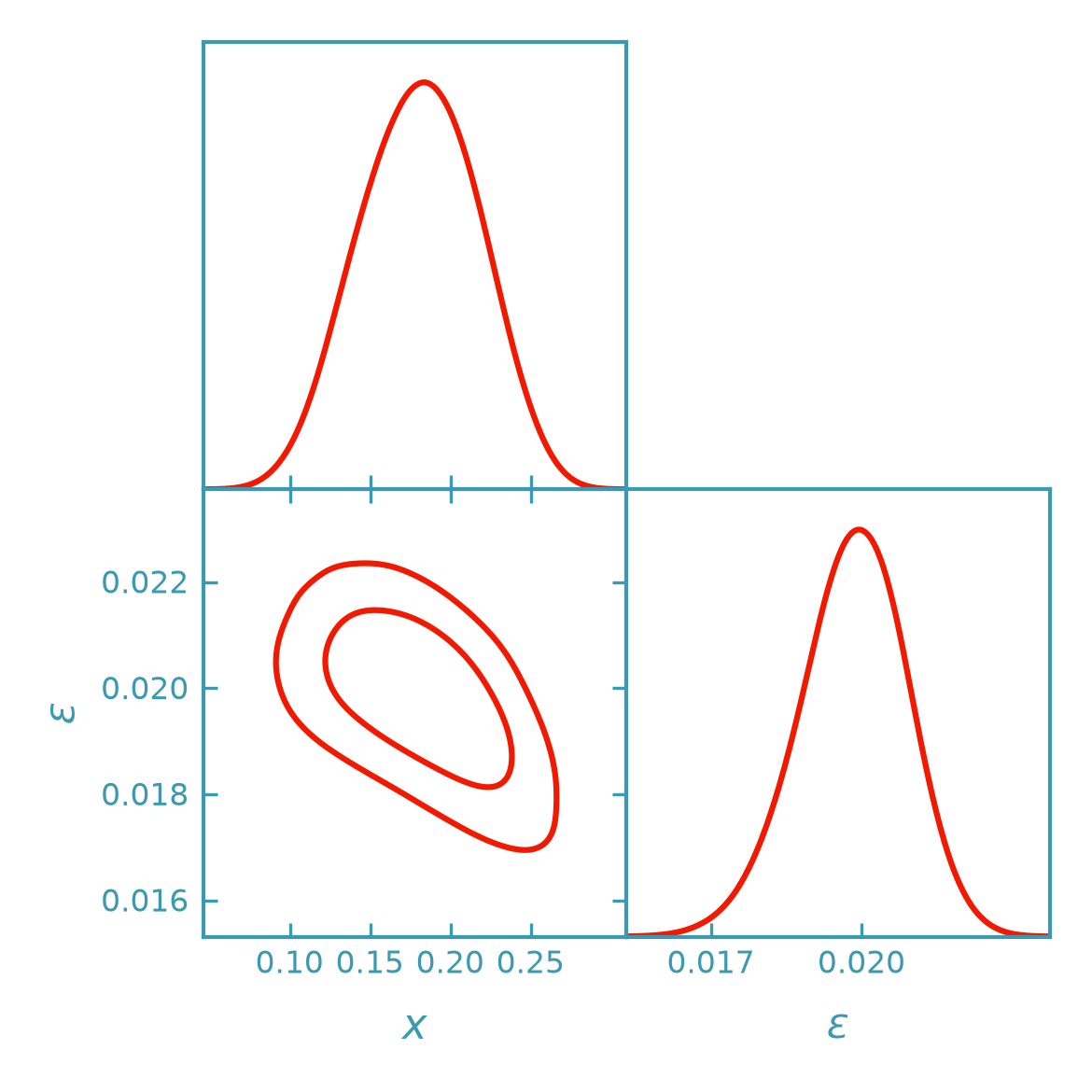
Sampling the DALI posterior with emcee

>>> import numpy as np
>>> from getdist import plots as getdist_plots
>>> from derivkit.forecast_kit import ForecastKit
>>> from derivkit.forecasting.getdist_dali_samples import dali_to_getdist_emcee
>>> def model_2d(theta):
...     # Nonlinear forward model with a curved parameter degeneracy
...     # (informally referred to as a "banana"-shaped posterior).
...     x, eps = float(theta[0]), float(theta[1])
...     k = 3.0
...     a = 4.0
...     c = 6.0
...     o1 = 1e2 * np.exp((x - k * eps) ** 2) * np.exp(a * eps)
...     o2 = 4e1 * np.exp(0.5 * x) * (1.0 + 0.3 * eps + c * (eps**3))
...     return np.array([o1, o2], dtype=float)
>>> theta0 = np.array([0.18, 0.02], dtype=float)
>>> cov = np.array([[1.0, 0.95],
...                 [0.95, 1.0]], dtype=float)
>>> fk = ForecastKit(function=model_2d, theta0=theta0, cov=cov)
>>> fisher = fk.fisher()
>>> g_tensor, h_tensor = fk.dali()
>>> samples = dali_to_getdist_emcee(
...     theta0=theta0,
...     fisher=fisher,
...     g_tensor=g_tensor,
...     h_tensor=h_tensor,
...     names=["x", "eps"],
...     labels=[r"x", r"\epsilon"],
...     label="DALI (emcee)",
... )
>>> dk_red = "#f21901"
>>> dk_yellow = "#e1af00"
>>> line_width = 1.5
>>> plotter = getdist_plots.get_subplot_plotter(width_inch=3.9)
>>> plotter.settings.linewidth_contour = line_width
>>> plotter.settings.linewidth = line_width
>>> plotter.settings.figure_legend_frame = False
>>> plotter.settings.legend_rect_border = False
>>> plotter.triangle_plot(
...     [samples],
...     params=["x", "eps"],
...     filled=False,
...     contour_colors=[dk_red],
...     contour_lws=[line_width],
...     contour_ls=["-"],
... )
>>> samples.numrows > 0
True

(png)

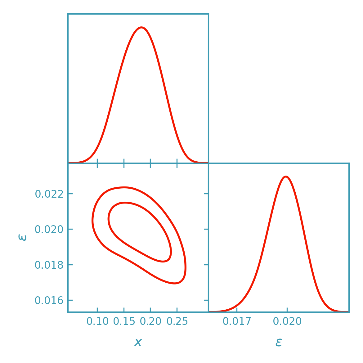
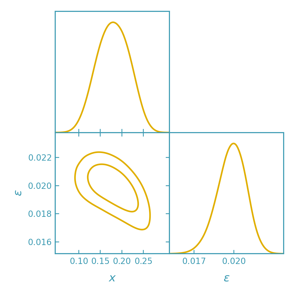
Sampling the DALI posterior with importance sampling

>>> import numpy as np
>>> from getdist import plots as getdist_plots
>>> from derivkit.forecast_kit import ForecastKit
>>> from derivkit.forecasting.getdist_dali_samples import dali_to_getdist_importance
>>> def model_2d(theta):
...     # Nonlinear forward model with a curved parameter degeneracy
...     # (informally referred to as a "banana"-shaped posterior).
...     x, eps = float(theta[0]), float(theta[1])
...     k = 3.0
...     a = 4.0
...     c = 6.0
...     o1 = 1e2 * np.exp((x - k * eps) ** 2) * np.exp(a * eps)
...     o2 = 4e1 * np.exp(0.5 * x) * (1.0 + 0.3 * eps + c * (eps**3))
...     return np.array([o1, o2], dtype=float)
>>> theta0 = np.array([0.18, 0.02], dtype=float)
>>> cov = np.array([[1.0, 0.95],
...                 [0.95, 1.0]], dtype=float)
>>> fk = ForecastKit(function=model_2d, theta0=theta0, cov=cov)
>>> fisher = fk.fisher()
>>> g_tensor, h_tensor = fk.dali()
>>> samples = dali_to_getdist_importance(
...     theta0=theta0,
...     fisher=fisher,
...     g_tensor=g_tensor,
...     h_tensor=h_tensor,
...     names=["x", "eps"],
...     labels=[r"x", r"\epsilon"],
...     label="DALI (importance)",
...     n_samples=80_000,
...     seed=0,
...     kernel_scale=1.3,
... )
>>> dk_yellow = "#e1af00"
>>> line_width = 1.5
>>> plotter = getdist_plots.get_subplot_plotter(width_inch=3.9)
>>> plotter.settings.linewidth_contour = line_width
>>> plotter.settings.linewidth = line_width
>>> plotter.settings.figure_legend_frame = False
>>> plotter.settings.legend_rect_border = False
>>> plotter.triangle_plot(
...     [samples],
...     params=["x", "eps"],
...     filled=False,
...     contour_colors=[dk_yellow],
...     contour_lws=[line_width],
...     contour_ls=["-"],
... )
>>> samples.numrows > 0
True

(png)

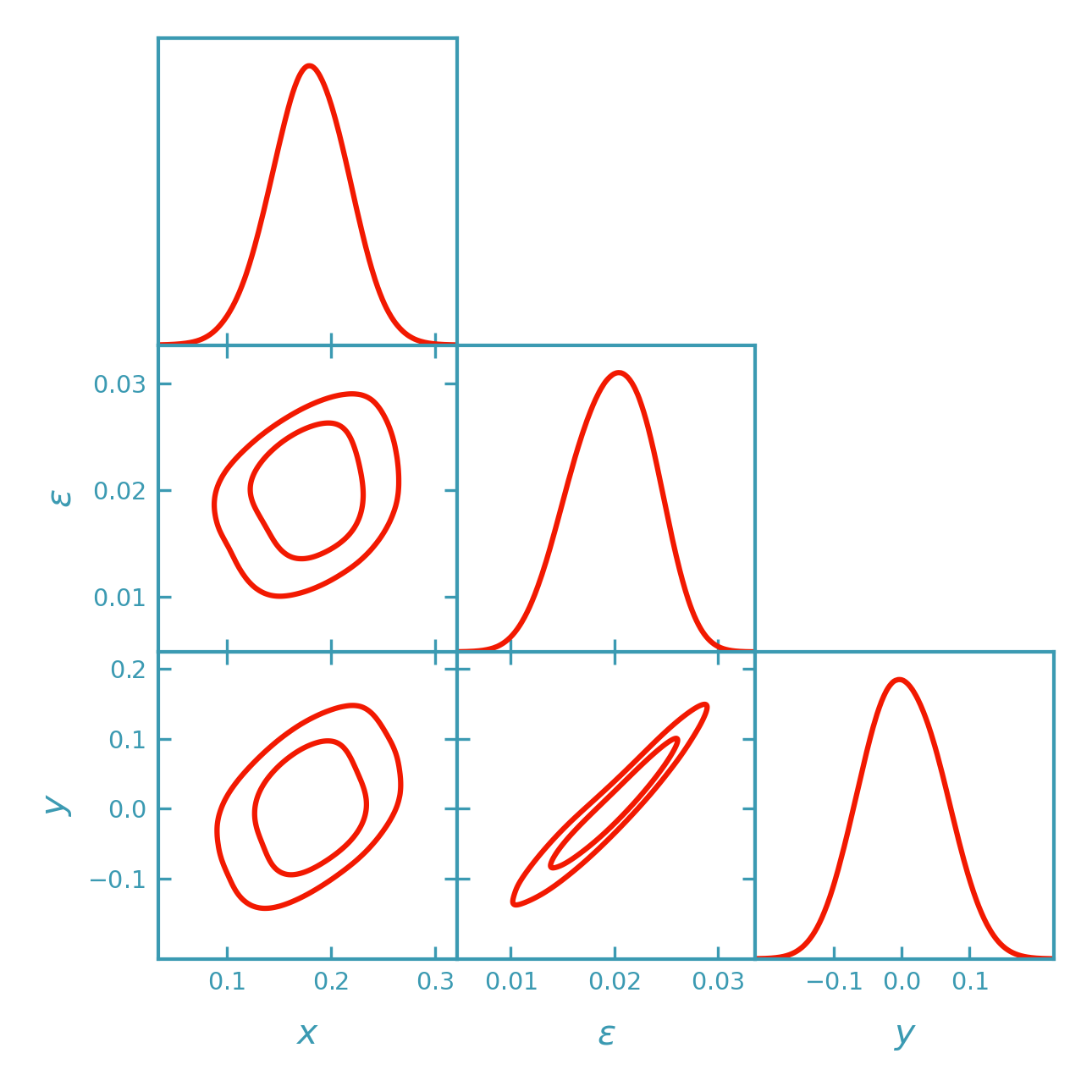
Three-parameter nonlinear example (emcee)

This section extends the 2D example to three parameters theta = [x, eps, y]. The forward model is constructed to produce a nonlinear posterior with pronounced parameter degeneracies. An additional coupling to y introduces further structure while preserving the dominant nonlinear features.

• o1 uses (x - k*eps - q*y)^2 to preserve the curved ridge in (x, eps) while introducing structure in (x, y) and (eps, y).

• o2 adds a mild dependence on y through an exponential prefactor.

>>> import numpy as np
>>> from getdist import plots as getdist_plots
>>> from derivkit.forecast_kit import ForecastKit
>>> from derivkit.forecasting.getdist_dali_samples import dali_to_getdist_emcee
>>> def model_3d(theta):
...     # A nonlinear model with 3 parameters:
...     x, eps, y = float(theta[0]), float(theta[1]), float(theta[2])
...     k = 3.0
...     q = 0.7
...     a = 4.0
...     c = 6.0
...     r = 0.25
...     o1 = 1e2 * np.exp((x - k * eps - q * y) ** 2) * np.exp(a * eps)
...     o2 = 4e1 * np.exp(0.5 * (x + r * y)) * (1.0 + 0.3 * eps + c * (eps**3))
...     return np.array([o1, o2], dtype=float)
>>> theta0 = np.array([0.18, 0.02, 0.00], dtype=float)
>>> cov = np.array([[1.0, 0.95],
...                 [0.95, 1.0]], dtype=float)
>>> prior_bounds = [(-0.4, 0.8), (-0.25, 0.25), (-0.4, 0.4)]
>>> fk = ForecastKit(function=model_3d, theta0=theta0, cov=cov)
>>> fisher = fk.fisher()
>>> g_tensor, h_tensor = fk.dali()
>>> samples = dali_to_getdist_emcee(
...     theta0=theta0,
...     fisher=fisher,
...     g_tensor=g_tensor,
...     h_tensor=h_tensor,
...     names=["x", "eps", "y"],
...     labels=[r"x", r"\epsilon", r"y"],
...     label="DALI (emcee, 3D)",
...     prior_bounds=prior_bounds,
... )
>>> dk_red = "#f21901"
>>> dk_yellow = "#e1af00"
>>> dk_blue = "#3b9ab2"
>>> line_width = 1.5
>>> plotter = getdist_plots.get_subplot_plotter(width_inch=4.3)
>>> plotter.settings.linewidth_contour = line_width
>>> plotter.settings.linewidth = line_width
>>> plotter.settings.figure_legend_frame = False
>>> plotter.settings.legend_rect_border = False
>>> plotter.triangle_plot(
...     [samples],
...     params=["x", "eps", "y"],
...     filled=False,
...     contour_colors=[dk_red, dk_blue, dk_yellow],
...     contour_lws=[line_width, line_width, line_width],
...     contour_ls=["-", "-", "-"],
... )
>>> samples.numrows > 0
True

(png)

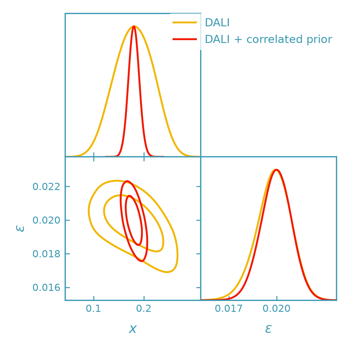
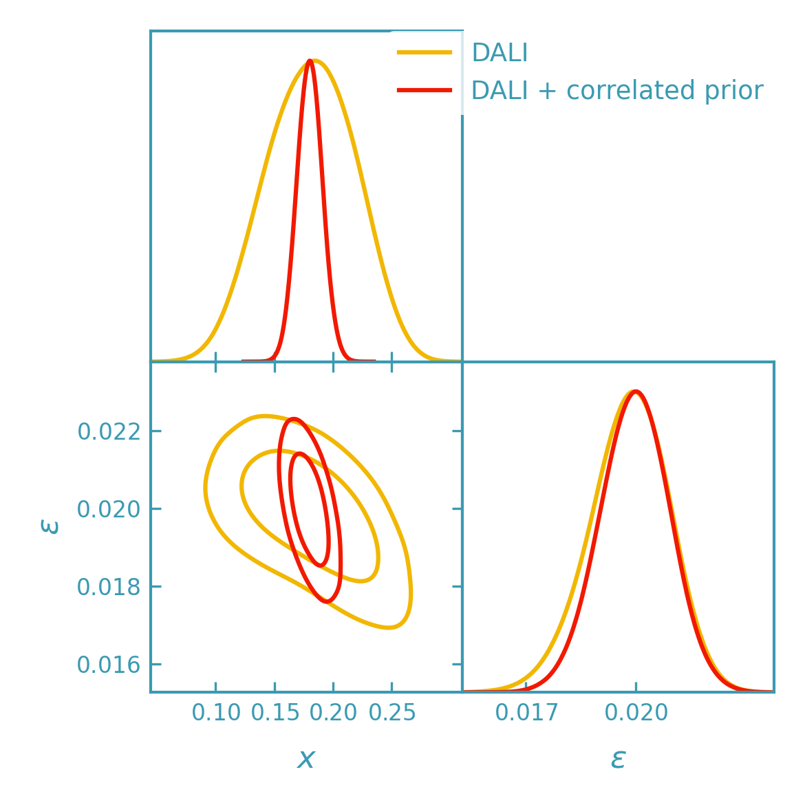
Including priors in DALI contours

Priors can be included in DALI sampling by passing them directly to the DerivKit GetDist helpers via prior_terms and/or prior_bounds. These are evaluated as part of the DALI log-posterior during sampling.

Sampler bounds mainly truncate the sampled region, while informative priors (especially correlated multivariate priors) can change the shape and orientation of the contours.

>>> import numpy as np
>>> from getdist import plots as getdist_plots
>>> from derivkit.forecast_kit import ForecastKit
>>> from derivkit.forecasting.getdist_dali_samples import dali_to_getdist_emcee
>>> def model_2d(theta):
...     x, eps = float(theta[0]), float(theta[1])
...     k = 3.0
...     a = 4.0
...     c = 6.0
...     o1 = 1e2 * np.exp((x - k * eps) ** 2) * np.exp(a * eps)
...     o2 = 4e1 * np.exp(0.5 * x) * (1.0 + 0.3 * eps + c * (eps**3))
...     return np.array([o1, o2], dtype=float)
>>> theta0 = np.array([0.18, 0.02], dtype=float)
>>> cov = np.array([[1.0, 0.95],
...                 [0.95, 1.0]], dtype=float)
>>> fk = ForecastKit(function=model_2d, theta0=theta0, cov=cov)
>>> fisher = fk.fisher()
>>> g_tensor, h_tensor = fk.dali()
>>> # Baseline: no priors
>>> samples_base = dali_to_getdist_emcee(
...     theta0=theta0,
...     fisher=fisher,
...     g_tensor=g_tensor,
...     h_tensor=h_tensor,
...     names=["x", "eps"],
...     labels=[r"x", r"\epsilon"],
...     label="DALI",
... )
>>> # With priors: wide bounds + a correlated multivariate Gaussian prior
>>> prior_bounds = [(-1.5, 1.5), (-0.8, 0.8)]
>>> # Strong correlated prior centered near theta0
>>> mu = np.array([0.18, 0.02], dtype=float)
>>> sx, seps, rho = 0.03, 0.006, -0.95
>>> cov_prior = np.array(
...     [[sx * sx,        rho * sx * seps],
...      [rho * sx * seps, seps * seps]],
...     dtype=float,
... )
>>> prior_terms = [("gaussian", {"mean": mu, "cov": cov_prior})]
>>> samples_prior = dali_to_getdist_emcee(
...     theta0=theta0,
...     fisher=fisher,
...     g_tensor=g_tensor,
...     h_tensor=h_tensor,
...     names=["x", "eps"],
...     labels=[r"x", r"\epsilon"],
...     label="DALI + correlated prior",
...     prior_bounds=prior_bounds,
...     prior_terms=prior_terms,
... )
>>> dk_red = "#f21901"
>>> dk_yellow = "#f2b701"
>>> line_width = 1.5
>>> plotter = getdist_plots.get_subplot_plotter(width_inch=3.9)
>>> plotter.settings.linewidth_contour = line_width
>>> plotter.settings.linewidth = line_width
>>> plotter.settings.figure_legend_frame = False
>>> plotter.settings.legend_rect_border = False
>>> plotter.triangle_plot(
...     [samples_base, samples_prior],
...     params=["x", "eps"],
...     filled=[False, False],
...     contour_colors=[dk_yellow, dk_red],
...     contour_lws=[line_width, line_width],
...     contour_ls=["-", "-"],
... )
>>> (samples_base.numrows > 0) and (samples_prior.numrows > 0)
True

(png)

Notes and conventions

• The non-Gaussianity here comes from the nonlinear forward model.

• getdist.MCSamples.loglikes stores minus the log-posterior (up to an additive constant), following GetDist conventions.

• Importance sampling uses a Fisher–Gaussian proposal; kernel_scale controls its width. If weights become extremely uneven, try increasing the scale slightly.

• Importance sampling is intended for fast visualization and exploratory work, and is reliable when the Fisher–Gaussian proposal closely matches the DALI posterior.

• For science analyses requiring a robust exploration of the posterior, including non-Gaussian structure and tails, we recommend using emcee to sample the DALI-expanded posterior.

Typical workflow

1. Compute Fisher F and higher-order tensors (G, H) with ForecastKit.

2. Use importance sampling for fast visualization and iteration.

3. Switch to emcee when robustness is required or strong non-Gaussianity leads to unstable importance weights.

4. Visualize and compare results using GetDist triangle plots.

See also

• derivkit.forecast_kit.ForecastKit

• derivkit.forecasting.dali.build_dali()

• derivkit.forecasting.expansions.logposterior_dali()

• derivkit.forecasting.getdist_dali_samples.dali_to_getdist_emcee()

• derivkit.forecasting.getdist_dali_samples.dali_to_getdist_importance()